Category Archives: hand-on activity (difficult)

Accidental double-diffusive mixing

When setting up the stratification for the Nansen “dead water” demo (that we’ll show later today, and until then I am not allowed to share any videos, sorry!), I went into a meeting after filling in layer 4 (the then lowest). When I came back, I wanted to fill in layer 5 as the new bottom layer. For this experiment we want the bottom four layers to have the same density (so we would actually only have one shallow top layer and then a deep layer below [but we can’t make enough salt water at a time for that layer, so I had to split it into four portions]), and I had mixed it as well as I could. But two things happened: a) my salinity was clearly a little fresher than the previous layer, and b) the water in the tank had warmed up and the new water I was adding with layer 5 was cold tap water. So I accidentally set up the stratification for salt fingering: warm and salty over cold and fresh! Can you spot the darker pink fingers reaching down into the slightly lighter pink water? How cool is this??? I am completely flashed. Salt fingering in a 6 meter long tank! :-D


The one where it would help to understand the theory better (but still: awesome tank experiment!)

The main reason why we went to all the trouble of setting up a quasi-continuous stratification to pull our mountain through instead of sticking to the 2 layer system we used before was that we were expecting to see a tilt of the axis of the propagating phase. We did some calculations of the Brunt-Väisälä frequency, that needs to be larger than the product of the length of the obstacle and the speed the obstacle is towed with (and it was, by almost two orders of magnitude!), but happy with that result, we didn’t bother to think through all the theory.

And what happened was what always happens when you just take an equation and stick the numbers in and then go with that: Unfortunately, you realize you should have thought it through more carefully.

Luckily, Thomas chose exactly that time to come pick me up for a coffee (which never happened because he got sucked into all the tank experiment excitement going on), and he suggested that having one mountain might not be enough and that we should go for three sines in a row.

Getting a new mountain underneath an existing stratification is not easy, so we decided to go for the inverse problem and just tow something on the surface rather than at the bottom. And just to be safe we went with almost four wavelengths… And look at what happens!

We are actually not quite sure if the tilting we observed was due to a slightly wobbly pulling of the — let’s use the technical term and go for “thingy”? — or because of us getting the experiment right this time, but in any case it does look really cool, doesn’t it? And I’ll think about the theory some more before doing this with students… ;-)

Fictitious forces (3/5): Coriolis force — how we think it should be taught

So how do we teach about the Coriolis force? The following is a shortened version of an article that Pierre de Wet and I wrote when I was still in Bergen, check it out here.

The Coriolis demonstration

A demonstration observing a body on a rotating table from within and from outside the rotating system was run as part of the practical experimentation component of the “Introduction to Oceanography” semester course. Students were in the second year of their Bachelors in meteorology and oceanography at the Geophysical Institute of the University of Bergen, Norway. Similar experiments are run at many universities as part of their oceanography or geophysical fluid dynamics instruction.

Materials:

  • Rotating table with a co-rotating video camera (See Figure 1. For simpler and less expensive setups, please refer to “Possible modifications of the activity”)
  • Screen where images from the camera can be displayed
  • Solid metal spheres
  • Ramp to launch the spheres from
  • Tape to mark positions on the floor
folie1

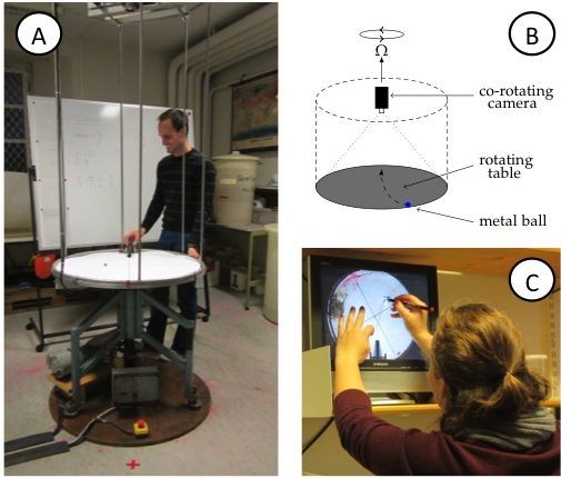
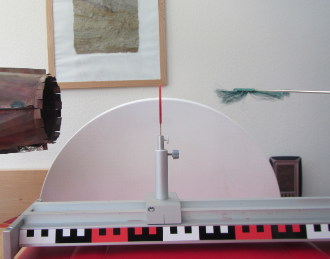
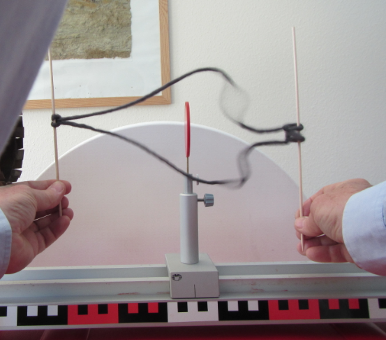
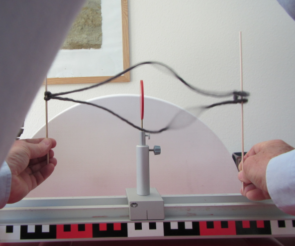
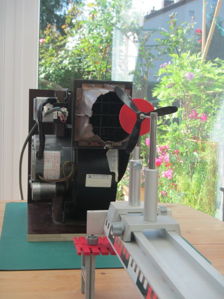
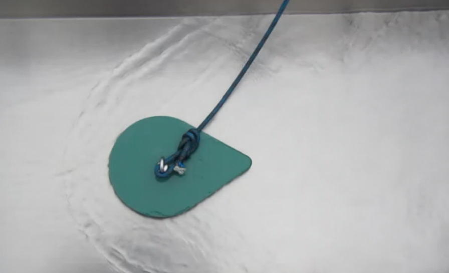
Figure 1A: View of the rotating table. Note the video camera on the scaffolding above the table and the red x (marking the catcher’s position) on the floor in front of the table, diametrically across from where, that very instant, the ball is launched on a ramp. B: Sketch of the rotating table, the mounted (co-rotating) camera, the ramp and the ball on the table. C: Student tracing the curved trajectory of the metal ball on a transparency. On the screen, the experiment is shown as filmed by the co-rotating camera, hence in the rotating frame of reference.


Time needed:

About 45 minutes to one hour per student group. The groups should be sufficiently small so as to ensure active participation of every student. In our small lab space, five has proven to be the upper limit on the number of students per group.

Student task:

In the demonstration, a metal ball is launched from a ramp on a rotating table (Figure 1A,B). Students simultaneously observe the motion from two vantage points: where they are standing in the room, i.e. outside of the rotating system of the table; and, on a screen that displays the table, as captured by a co-rotating camera mounted above it. They are subsequently asked to:

  • trace the trajectory seen on the screen on a transparency (Figure 1C),
  • measure the radius of this drawn trajectory; and
  • compare the trajectory’s radius to the theorized value.

The latter is calculated from the measured rotation rate of the table and the linear velocity of the ball, determined by launching the ball along a straight line on the floor.

Instructional approach

In years prior to 2012, the course had been run along the conventional lines of instruction in an undergraduate physics lab: the students read the instructions, conduct the experiment and write a report.

In 2012, we decided to include an elicit-confront-resolve approach to help students realize and understand the seemingly conflicting observations made from inside versus outside of the rotating system (Figure 2). The three steps we employed are described in detail below.

folie2

Figure 2: Positions of the ramp and the ball as observed from above in the non-rotating (top) and rotating (bottom) case. Time progresses from left to right. In the top plots, the position in inert space is shown. From left to right, the current position of the ramp and ball are added with gradually darkening colors. In the bottom plots, the ramp stays in the same position, but the ball moves and the current position is always displayed with the darkest color.

  1. Elicit the lingering misconception

1.a The general function of the “elicit” step

The goal of this first step is to make students aware of their beliefs of what will happen in a given situation, no matter what those beliefs might be. By discussing what students anticipate to observe under different physical conditions before the actual experiment is conducted, the students’ insights are put to the test. Sketching different scenarios (Fan (2015), Ainsworth et al. (2011)) and trying to answer questions before observing experiments are important steps in the learning process since students are usually unaware of their premises and assumptions. These need to be explicated and verbalized before they can be tested, and either be built on, or, if necessary, overcome. 

1.b What the “elicit” step means in the context of our experiment

Students have been taught in introductory lectures that in a counter-clockwise rotating system (i.e. in the Northern Hemisphere) a moving object will be deflected to the right. They are also aware that the extent to which the object is deflected depends on its velocity and the rotational speed of the reference frame.

A typical laboratory session would progress as follows: students are asked to observe the path of a ball being launched from the perimeter of the circular, not-yet rotating table by a student standing at a marked position next to the table, the “launch position”. The ball is observed to be rolling radially towards and over the center point of the table, dropping off the table diametrically opposite from the position from which it was launched. So far nothing surprising. A second student – the catcher – is asked to stand at the position where the ball dropped off the table’s edge so as to catch the ball in the non-rotating case. The position is also marked on the floor with insulation tape.

The students are now asked to predict the behavior of the ball once the table is put into slow rotation. At this point, students typically enquire about the direction of rotation and, when assured that “Northern Hemisphere” counter-clockwise rotation is being applied, their default prediction is that the ball will be deflected to the right. When asked whether the catcher should alter their position, the students commonly answer that the catcher should move some arbitrary angle, but typically less than 90 degrees, clockwise around the table. The question of the influence of an increase in the rotational rate of the table on the catcher’s placement is now posed. “Still further clockwise”, is the usual answer. This then leads to the instructor’s asking whether a rotational speed exists at which the student launching the ball, will also be able to catch it him/herself. Ordinarily the students confirm that such a situation is indeed possible.


  1. Confronting the misconception

2.a The general function of the “confront” step

For those cases in which the “elicit” step brought to light assumptions or beliefs that are different from the instructor’s, the “confront” step serves to show the students the discrepancy between what they stated to be true, and what they observe to be true.

2.b What the “confront” step means in the context of our experiment

The students’ predictions are subsequently put to the test by starting with the simple, non-rotating case: the ball is launched and the nominated catcher, positioned diametrically across from the launch position, seizes the ball as it falls off the table’s surface right in front of them. As in the discussion beforehand, the table is then put into rotation at incrementally increasing rates, with the ball being launched from the same position for each of the different rotational speeds. It becomes clear that the catcher need not adjust their position, but can remain standing diametrically opposite to the student launching the ball – the point where the ball drops to the floor. Hence students realize that the movement of the ball relative to the non-rotating laboratory is unaffected by the table’s rotation rate.

This observation appears counterintuitive, since the camera, rotating with the system, shows the curved trajectories the students had expected; circles with radii decreasing as the rotation rate is increased. Furthermore, to add to their confusion, when observed from their positions around the rotating table, the path of the ball on the rotating table appears to show a deflection, too. This is due to the observer’s eye being fooled by focusing on features of the table, e.g. cross hairs drawn on the table’s surface or the bars of the camera scaffold, relative to which the ball does, indeed, follow a curved trajectory. To overcome this latter trickery of the mind, the instructor may ask the students to crouch, diametrically across from the launcher, so that their line of sight is aligned with the table’s surface, i.e. at a zero zenith angle of observation. From this vantage point the ball is observed to indeed be moving in a straight line towards the observer, irrespective of the rate of rotation of the table.

To further cement the concept, the table may again be set into rotation. The launcher and the catcher are now asked to pass the ball to one another by throwing it across the table without it physically making contact with the table’s surface. As expected, the ball moves in a straight line between the launcher and the catcher, who are both observing from an inert frame of reference. However, when viewing the playback of the co-rotating camera, which represents the view from the rotating frame of reference, the trajectory is observed as curved.

  1. Resolving the misconception

3.a The general function of the “resolve” step

Misconceptions that were brought to light during the “elicit” step, and whose discrepancy with observations was made clear during the “confront” step, are finally corrected in the “resolve” step. While this sounds very easy, in practice it is anything but. The final step of the elicit-confront-resolve instructional approach thus presents the opportunity for the instructor to aid students in reflecting upon and reassessing previous knowledge, and for learning to take place.

3.b What the “resolve” step means in the context of our experiment

The instructor should by now be able to point out and dispel any remaining implicit assumptions, making it clear that the discrepant trajectories are undoubtedly the product of viewing the motion from different frames of reference. Despite the students’ observations and their participation in the experiment this is not a given, nor does it happen instantaneously. Oftentimes further, detailed discussion is required. Frequently students have to re-run the experiment themselves in different roles (i.e. as launcher as well as catcher) and explicitly state what they are noticing before they trust their observations.

Possible modifications of the activity:

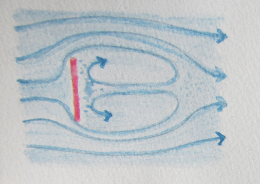
We used the described activity to introduce the laboratory activity, after which the students had to carry out the exercise and write a report about it. Follow-up experiments that are often conducted usually include rotating water tanks to visualize the effect of the Coriolis force on the large-scale circulation of the ocean or atmosphere, for example on vortices, fronts, ocean gyres, Ekman layers, Rossby waves, the General circulation and many other phenomena (see for example Marshall and Plumb (2007)).

Despite their popularity in geophysical fluid dynamics instruction at the authors’ current and previous institutions, rotating tables might not be readily available everywhere. Good instructions for building a rotating table can, for example, be found on the “weather in a tank” website, where there is also the contact information to a supplier given: http://paoc.mit.edu/labguide/apparatus.html. A less expensive setup can be created from old disk players or even Lazy Susans. In many cases, setting the exact rotation rate is not as important as having a qualitative difference between “fast” and “slow” rotation, which is very easy to realize. In cases where a co-rotating camera is not available, by dipping the ball in either dye or chalk dust (or by simply running a pen in a straight line across the rotating surface), the trajectory in the rotating system can be visualized. The method described in this manuscript is easily adapted to such a setup.

Lastly we suggest using an elicit-confront-resolve approach even when the demonstration is not run on an actual rotating table. Even if the demonstration is only virtually conducted, for example using Urbano & Houghton (2006)’s Coriolis force simulation, the approach is beneficial to increasing conceptual understanding.

Using the Monash Simple Climate Model as first exposure to “real” climate models

When talking to the “general public” (which sometimes just means friends or relatives) about working in climate sciences, it is sometimes really difficult to explain what it is we do every day. I have described a very simple way of explaining how climate models work before. But while this might help provide a general idea of what a model does, it does not show us what climate models actually do. But there is a great tool out there that does exactly that!

The Monash simple climate model is a real climate model. When I was still in Kiel, almost 10 years ago, my sailing buddy Janine was working on implementing the first version of that model! And now the DKRZ (the German Climate Computing Center) hosts an web-based interface that lets anyone access the model.

You can build up the climate model step by step, adding representations of processes like ice albedo, clouds, or many other and then compare model runs including those processes with those runs without. You are even shown the difference between those two runs to see how properties like surface temperatures are affected by the process under investigation! And really awesome feature? The visualization of which processes are switched on and off. See below: On the left, in experiment A, all processes are switched on (and therefore shown in the picture on the top left). In Experiment B, on the right, almost all processes have been switched off, only incoming solar radiation and outgoing radiation are active. Looking at the temperatures below, this shows how Experiment B is only influenced by the sun and temperatures are the same along lines of constant latitude. In Experiment A, though, the temperatures are modified by many more processes, and therefore the distribution is a lot more messy.

Screen Shot 2016-02-24 at 14.39.55

Screenshot from http://mscm.dkrz.de, shared under CC BY-NC-SA

You can also look at different climate change scenarios, and you always get to see the CO2 forcing of the respective scenario. You can also compare scenarios with each other (see below). Doing this, you can vary parameters, too, to investigate their impact. You can always look at different model fields like surface and subsurface ocean temperatures, atmospheric temperatures, atmospheric water vapor or snow/ice cover.

Screen Shot 2016-02-24 at 14.52.44

Screenshot from http://mscm.dkrz.de, shared under CC BY-NC-SA

There are very nice video tutorials for a quick start, and puzzles where you can test how well you understand the model.

I absolutely love this tool, and I wish I was teaching anything related to ocean and climate so I could use it in my teaching. This opens up so many possibilities for inquiry-based learning. Or basically just interest-driven exploration, which would be so fun to initiate and then support! You should definitely check it out! http://mscm.dkrz.de/

Visualizing flow around a paddle

Whenever I’m in a canoe or kayak, I love watching the two eddies that form behind the paddle when you pull it through the water. It looks kinda like this:

Screen shot 2015-06-27 at 4.03.20 PM

Flow around a paddle

Instead of pulling a paddle through more or less stagnant water, we could also use a stationary paddle in a flow. And that is the setup I want to discuss today: A stationary, round paddle perpendicular to an air flow.

A very cool feature of the paddle – which we know has to exist from the sketch above – is shown below: There is a point somewhere downstream of the paddle, where the direction of the air flow changes and a return flow towards the paddle starts. You can see that the threads on the stick I am placing in the return flow go partly towards, partly away from the paddle. So clearly the stick is in the right spot!

IMG_1887

Visualizing the flow field behind a paddle with a threaded stick

Another visualization that my dad came up with below: Threads are pulled back towards the paddle in the return flow.

IMG_1890

Visualizing the return flow behind a paddle with threads

Doesn’t it look awesome?

IMG_1891

Visualizing the return flow behind a paddle with threads

Another way to visualize the change in flow direction is to take a rotor and move it from far downstream of the paddle towards the paddle and back.

IMG_1931

Visualizing the change in flow direction by moving a rotor towards and away from a paddle blocking an air stream

All of this is shown in the movie:

Don’t you wish you had all this stuff to play with? :-)

(And do you now understand why I was so excited about the diving duck? :-))

Wave fields around objects in a channel

One of the reasons I have been wanting to do the vortex street experiment I wrote about on Monday is that it is pretty difficult to visualize flow fields (especially if you neither want to pollute running water somewhere in nature, nor want to waste a lot of water by setting up the flow yourself). As a first order approximation, pulling an object through a stagnant water body is the same as the water body moving past a stationary object.

At the Thinktank Birmingham, they do have a small channel with water constantly running through, and a couple of objects that you can place in the current. Unfortunately, what you see is the wave field that is caused by the obstacle, not the current field.

MVI_9288

Wave field developing around a body inserted into a channel

It is still pretty cool to play with it, though!

[vimeo 119838613]

But neither of the setups (the channel discussed above or the vortex streets on a plate thing from Monday) is really optimally suited to teaching students the way a flow field will react to an obstacle. How amazing would it be if we had a flow field that could be modified to suit our needs? Stay tuned – I might have a solution for you on Friday! :-)

Salt fingering

My absolute favorite experiment ever: salt fingering.

I know I’ve said it before about another experiment, even today, but this is my absolute favorite experiment and I still get endlessly fascinated. I’ve written about salt fingering before, and given tips on run the experiment, but today we tried a different setup.

We used the same tank as in the “influence of salinity and temperature on density“, put warm, dyed water on the one side of the dam and cold fresh water on the other side.

Contrary to Rolf’s advice, we didn’t aim for specific temperatures and salinities to hit the density ratio in a specific way, but just went for really hot and really cold.

We pulled the parting out, and after a couple of minutes, salt fingers started to develop.

Unfortunately, they are really difficult to take pictures of.

But a lot of students watched and will hopefully remember what they saw.

And even if not – I thought it was awesome and Rolf said they were the best salt fingers he had seen yet – even though we just winged it ;-)

Hydraulic jump II

More movies of my kitchen sink.

I am really fascinated by the hydraulic jumps in my kitchen sink. I can’t believe I haven’t used this before when I was teaching! Yes, movies of rivers and rapids are always really impressive, too, but how cool is it to be able to observe hydraulic jumps in your own sink? Let me remind you:

Hydraulic jump in my kitchen sink. Video here

So this is what happens when the water jet hits the (more or less) level bottom of the sink. But what would happen if it instead hit a slope?

Now, if I wasn’t working a full-time job, or if that job wasn’t completely unrelated to anything to do with hydraulic jumps, I would now proudly present movies of all kinds of hydraulic jumps on sloped surfaces. As it is, I can tell you that I have tons of ideas of where to go to make really nice movies, but for now this is all I can offer:

Yes, that is a chopping board in a sink. It shows really nicely how the hydraulic jump occurs closer to the point of impact of the jet as you go uphill (because the water slows down faster going in that direction than going downhill) and again how the radius depends on the flow speed of the jet. Stay tuned for a more elaborate post on this!

Hydraulic jumps

Water changing its velocity from above to below the critical velocity.

Recently in beautiful Wetzlar: The river Lahn flows through the city below the medieval cathedral at sunset. And I’m showing you this because we can observe a hydraulic jump!

A hydraulic jump occurs when water that was flowing faster than the critical speed suddenly slows down to below the critical speed. Some of its kinetic energy is converted to potential energy (see the higher surface levels of the turbulent part of the fluid {except in this example the water is flowing down a steep slope, so the higher levels are a bit tricky to observe}) and a lot of energy is lost to turbulence. A very nice example can be seen here:

As the water moves away from where the jet hits the sink, it slows down. Can you spot the hydraulic jump? Isn’t it cool to watch how it is pushed away if the flow rate is higher, and how it comes back again when the tap is slowly closed?

P.S.: Yes, I’m being very vague about what that critical speed might be. Stay tuned for a post on that, I’m working on it! Just had to share the Lahn movie :-)

Hydrostatic pressure

What are students not understanding about hydrostatic pressure?

Tomorrow (today by the time this post will go online, I guess) I will present the paper “Identifying and addressing student difficulties with hydrostatic pressure” by Loverude, Heron and Kautz at the Journal Club at work. So tonight I am trying out a couple of experiments that I would like to show with it.

I already know that I am not supposed to show the experiments during the talk, but I figure that there is no harm in having them prepared in case anyone wants to see them afterwards.

And good thing I tried them before instead of just assuming that they would work!

For the first experiment, I had this awesome idea to re-create something I saw as a child when on vacation on a farm:

I was clearly very impressed with it – this picture is from 1994 and I remembered it and asked my parents to track it down for me!

Anyway. Since I wasn’t sure if my colleagues would be happy with that amount of water on the floor, I decided to go for a smaller version of the same thing.

This is what I wanted it to look like (and what it looks like in my presentation):

hydrostaticpressure01

Hydro(almost)static pressure in the idealized case.

And this is what the experiment ended up looking like:

How disappointing! I guess the holes that I poked into the bottle aren’t well made. But good thing I tried. Watch the movie if you want to pay attention to if you ever want to present this experiment.

Yes. You want to use tape that keeps the water inside the bottle. Until you want to take the tape off. Then you wish you had used something that actually comes off…… ;-)