Tag Archives: EDarelius&team

Tides themselves don’t induce (a lot of) mixing, only tides hitting topography do. An experiment.

As you might have noticed, the last couple of days I have been super excited to play with the large tanks at GFI in Bergen. But then there are also simple kitchen oceanography experiments that need doing that you can bring into your class with you, like for example one showing that tides and internal waves by themselves don’t do a lot of mixing, and that only when they hit topography the interesting stuff starts happening.

So what we need is a simple 2-layer system and two different cases: One with topography, one without. And because we want to use it to hand around in class, the stratification should be indestructible (-> oil and water) and the container should be fairly tightly sealed to prevent a mess.

Here we go:

There definitely is a lot to be said for kitchen oceanography, too! Would you have thought that using just two plastic bottles and some oil and water could give such a nice demonstration?

Waves in a density stratification. One of the most beautiful tank experiments I’ve ever seen.

It’s pretty impressive when a mountain moves through a stratification and generates lee waves. But what I find even more impressive: The waves that travel behind the mountain when the mountain is long gone. See here:

This kind of stuff looks more like a numerical simulation than something actually happening in a tank, doesn’t it? I am pretty stoked that we managed to set up such a nice stratification! Those are the things that make me really really happy :-)

(The setup of this experiment is the same as in this post)

Tank experiment: Lee waves in a fancy density (and dye) stratification

Did you seriously think we’d stop tank experiments with only 2-layer systems? Nooo!

Today, the plan was to set up a continuous stratification, which I have been planning to do for many years. After fiddling with the setup all morning (do you have any idea how many fittings on all kinds of hoses are needed to get that to work well?), reality set in and we ended up doing a quasi-continuous stratification, i.e. 12 density layers dyed in 6 different colors*.

And this is what it looks like when you tow a mountain through that stratification (and try to ignore the excited audience being reflected in the tank): Still very nice lee waves and surprisingly little turbulence!

*We set up the tank to contain the same amount of salt as our 2-layer system yesterday, so instead of one big density jump from about 1000g/l to 1026g/l, this now happened in 5 smaller, more or less regular, jumps. And here is how we did it in the end: Two large reservoirs (unfortunately of different diameters), one containing freshwater, the other one filled up to the same height, containing as much salt as we had in our experiment yesterday. Now the height of the reservoirs was divided in 12 equal dzs, and for each dz that went out of the “freshwater” tank into the experimental tank, we added salt water of the same dz to the “freshwater” tank, which thus continued to increase in salinity. The water that we mixed that way went through a hose and entered the experimental tank through the bottom of the tank through a hole over which we had put the mountain (to contain mixing to a small volume and also so we didn’t have to watch water shooting out of that hole in our nice stratification). So as the water we added became increasingly dense, it nicely layered itself underneath the other water in the tank. And we just had to add more and more dye for the color gradient. Easy peasy :-)

The one where it would help to understand the theory better (but still: awesome tank experiment!)

The main reason why we went to all the trouble of setting up a quasi-continuous stratification to pull our mountain through instead of sticking to the 2 layer system we used before was that we were expecting to see a tilt of the axis of the propagating phase. We did some calculations of the Brunt-Väisälä frequency, that needs to be larger than the product of the length of the obstacle and the speed the obstacle is towed with (and it was, by almost two orders of magnitude!), but happy with that result, we didn’t bother to think through all the theory.

And what happened was what always happens when you just take an equation and stick the numbers in and then go with that: Unfortunately, you realize you should have thought it through more carefully.

Luckily, Thomas chose exactly that time to come pick me up for a coffee (which never happened because he got sucked into all the tank experiment excitement going on), and he suggested that having one mountain might not be enough and that we should go for three sines in a row.

Getting a new mountain underneath an existing stratification is not easy, so we decided to go for the inverse problem and just tow something on the surface rather than at the bottom. And just to be safe we went with almost four wavelengths… And look at what happens!

We are actually not quite sure if the tilting we observed was due to a slightly wobbly pulling of the — let’s use the technical term and go for “thingy”? — or because of us getting the experiment right this time, but in any case it does look really cool, doesn’t it? And I’ll think about the theory some more before doing this with students… ;-)

Dead water — the fancy experiment including Nansen himself

Now that we do have a really awesome 12-layer 6-color stratification, we obviously had to do the dead water experiment again. This time we chose to include a not-too-happy-looking Nansen on the ship, too!

I love this even more than the one we did yesterday!

“Dead water” or: ship-generated internal waves

And here is another experiment that can be done with the same stratification as the lee waves: Towing a ship to explore the phenomenon of “dead water”!

Dead water is well known for anyone sailing on strong stratifications, i.e. in regions where there is a shallow fresh or brackish layer on top of a much saltier layer, e.g. the Baltic Sea of some fjords. It has been described as early as 1893 by Fridtjof Nansen, who wrote, sailing in the Arctic: “When caught in dead water Fram appeared to be held back, as if by some mysterious force, and she did not always answer the helm. In calm weather, with a light cargo, Fram was capable of 6 to 7 knots. When in dead water she was unable to make 1.5 knots. We made loops in our course, turned sometimes right around, tried all sorts of antics to get clear of it, but to very little purpose.” (cited in Walker,  J.M.; “Farthest North, Dead Water and the Ekman Spiral,” Weather, 46:158, 1991)

Finding the explanation for this phenomenon took a little while, but in 1904, Vilhelm Bjerknes explained that “in the case of a layer of fresh water resting on the top of salt water, a ship will not only produce the ordinary visible waves at the boundary between the water and the air, but will also generate invisible waves in the salt-water fresh-water boundary below” — a lot of the ship’s work is now going towards generating the internal waves at the interface rather than for propulsion.

It’s hard to imagine how a ship will generate waves somewhere in the water below, so we are demonstrating this in the tank:

Isn’t it fascinating to think about how far oceanography has come in only a little over a hundred years? And despite all the extremely powerful instrumentation and modelling that we have available now, how cool are even such simple demonstrations in a tank? These are the moments where I know exactly why I went to study oceanography in the first place, and why it’s still the most fascinating subject I can think of…

Lee waves in the tank

Did you guess what we needed the stratification for? Yes — we are moving mountains again! :-)

What we want to look at: How a current reacts to an obstacle in its way, especially a current in a stratification. But since it is really difficult to set up a current in a tank, let alone a stratified one, we are doing the next best thing: Moving the obstacle relative to the water rather than the other way round.

And this is what it looks like:

Et voilà: Beautiful lee waves!

And look at the paper bits floating on the surface and how they visualize convergences and divergences in the upper layer!

The three layers in the pink all have (more or less) similar densities, and are only dyed slightly differently because we had to make several batches of dyed salt water to be able to fill the tank. But look how well they show that the wave is really happening at the interface, and that the other layers are phase locked. What would happen if the stratification inside the pink layer was stronger? Just wait and see…. ;-)

Kelvin-Helmholtz instabilities

I’m back at my happy place — the teaching lab at GFI in Bergen! :-)

Here a quick look at what we’ve been doing today: Filling the large wave tank! With clear fresh water and then salty pink water that forms a layer below. As the pink water flows underneath the clear water, there is shear between the two layers, waves form and then they break. Beautiful Kelvin-Helmholtz shear instabilities!

Why have we filled the large tank? Just you wait and see… ;-)

We discovered a new galaxy! Or at least a very pretty vortex

When we move our wall back and forth, we create very strong wing tip vortices that persist for quite a long time.

Above, you see the vortex, lit by a laser sheet close to the surface. You can see the whole column rotating as one, that bright smudge below the swirl is the lower part of the column. There are so many of our neutrally buoyant particles in there that the column looks bright even though it isn’t directly lit by the laser.

And in the picture above, you see those bright smudges on the left of the picture? That’s particles that the vortex hoovered up and then dumped in its path, pretty much like a hurricane would.

And that’s what it looks like as a gif:

“No one believes a theory, except the theorist. Everyone believes an experiment — except the experimenter.”

Different types of experiments, and why we use such a weirdly-shaped “Antarctica” and are happy with it.

When we want to show people images of our model experiments in a tank, people often imagine that they will be shown cute little miniature landscapes, looking much like the ones you see for really fancy model train setups. And then they are hugely disappointed when they see pictures like the one below and we tell them that yes! that’s our Antarctica that Nadine is climbing on, while Elin is sitting in the Southern Ocean.

The kind of experiment everybody hopes to see could, according to Faller (1981), be classified as a simulation: representing the natural world in miniature, including every detail. Data from those experiments — since they would in theory be realistic representations of the real world — could be used to fill in missing data from the real world in regions that are hard to get real data from, like for example the Southern Ocean. However, since those experiments are designed to represent the complexity of the real world, interpretation of the experiments is as complex as it is to interpret data from the real world: There are so many processes involved that it is hard to isolate effects of individual processes.

The kind of experiments we are doing would be classified as abstractions. Faller describes this kind of experiment as similar to abstract art: Only the main features, or better: the artist’s interpretation of the main features, are reproduced and everything else is omitted. That makes the art difficult to understand for anyone who isn’t well versed in abstract art, but for the experts it is obvious what the point is.

In case of our experiments that means that we have all the relevant features, or better: our interpretation of what we believe to be relevant features, of Antarctica present in the tank: the parts of topography that we think have an influence on how the current should behave, i.e. a V-shaped canyon, a source that supplies water of the correct properties into the ambient “ocean” water, an ice shelf. And when that ice shelf is tilted, we feel like our experiments are already becoming pretty realistic!

These abstractions are the kinds of experiments in which you can, because they are relatively simple, develop new theories when new features of the circulation emerge that you then have to rationalize and include in your theories after the fact.

We have actually also done another type of experiment, a verification. I wrote about it in this post: we tilted the ice shelf because this is a case for which we actually knew from theory how our current should behave, in contrast to all the previous experiments where we didn’t actually know what to expect, and we were happy when we observed exactly what we expected based on theoretical considerations. So in this case the experiment wasn’t about discovering something new, but rather making sure that our understanding of theory and what goes on in the tank actually match.

Faller describes a last type of experiment: the extension. That is the kind of experiment that you could perform after a successful verification experiment: Pushing the boundaries of the theory. Does it still hold if the current introduced in the tank is very fast or very slow? If the water is very deep? If the slope of the ice shelf is very large or small? Basically, every parameter could now be changed until we know for which cases the theory holds, and for which it does not.

So why am I writing all of this today? Faller’s (1981) article, before he goes on to describe the framework to think about geophysical fluid dynamics experiments that I mentioned above and which I find quite helpful to consider, starts with the sentence “No one believes a theory, except the theorist. Everyone believes an experiment — except the experimenter.” On this blog, our goal is to bring the two together and not make anyone believe either of them, but to show how both can work together to mutual benefit.

Faller, A. J. (1981). The origin and development of laboratory models and analogues of the ocean circulation. Evolution of Physical Oceanography, 462-479.