If you can sketch it, you can explain it!
This is supplementary material to Daae & Glessmer (2022), written by Kjersti Daae. We present the sketching exercise for fjord circulation (Example 1 in the article) in more detail. This is an exercise we do in a bachelor level course “Physics of the Atmosphere and Ocean” at the Geophysical Institute, University of Bergen. The students are from two different study programmes (Bachelor’s Programme in Climate, Atmosphere and Ocean Physics, 3rd semester, and Energy, Integrated Master’s, 5thsemester). The course is taught in a flipped classroom style, with a mix of targeted mini-lectures and group exercises where students participate actively. We typically have around 15-30 students in the course, and the teaching takes place in classrooms intended for group work (i.e., roundtables for groups of 3-6 students, with separate screens).
Fjord circulation sketching task
Fjord circulation, also known as estuarine circulation, describes the circulation in an estuary or a fjord, driven by freshwater sources and sinks. To understand the concept and being able to make calculations of such systems, students need to understand which freshwater fluxes are at play and the concepts of conservation of volume and mass.
Preparations
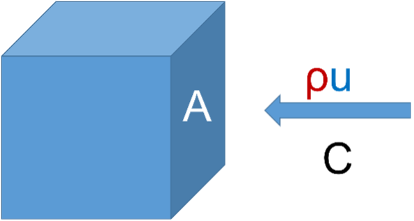
We typically start off by making sure students understand the definitions of transports and fluxes. They read theory about this topic as preparation for the class, but often need to repeat and discuss this during class to fully understand the definitions. Transport and flux are defined as
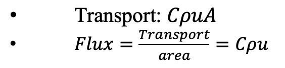 Where is the concentration of “something” (salt, oxygen, heat, etc), ρ is the sea water density, u is the current speed and A is the cross-section area we are interested in.
The students work in groups to fill in the expressions for the transports below, i.e., to find the correct parameters and units.
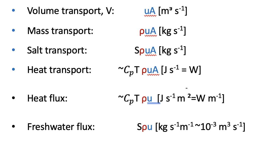
The salt transport is usually the easiest to fill in since it follows directly from the definition above. They simply need to replace the C with the salinity. The students may need some help to figure out the units, though, since they need to implement the conversion 1 m3s-1 = 1000 kg s-1.
The mass and volume transports are a bit trickier, since they cannot simply replace the C, but needs to understand what is transported.
For the heat transport, most students include temperature, but understand that something is not quite right from the unit analysis. Here they need the specific heat capacity, Cp, to arrive at the correct expression and units. We find it helpful to clearly state ‘heat transport’ and not use the term ‘temperature’ in this exercise. When we discuss in plenum afterwards, we emphasize that when we talk about heat, we always include the specific heat capacity Cp.
Sketching exercise
When the students get a hang on the definitions of transports and fluxes, we dive into the sketching of the fjord circulation. The exercise is divided into many small steps to guide the students. We typically give the groups 1-2 exercise instructions at a time to make sure they focus on each task instead of rushing towards the end. We also stop and discuss some tasks in plenum when there are interesting questions from the students or they sketch something worth sharing in plenum. For instance, students sometimes get creative when sketching freshwater fluxes and include sea ice freezing and melting or glacier calving. This leads to good discussions on seasonal and geographical variations in the freshwater fluxes. When sketching the flow regime, students sometimes include tides and wind-forced flow, which are also great topics for further discussions and comparisons with the fjord circulation. Usually, we ask the students to leave these out for this exercise, but promise to return to these processes. In the follow-up exercises where they make estimates of volume transports and current speeds in specific fjords they can compare the fjord circulation current speeds with typical tidal currents and wind-forced currents.
Instructions
- Sketch a transect of a fjord, from the fjord mouth to the fjord head. Annotate the sketch to indicate topographical features
- Discuss relevant sources and sinks for freshwater in the fjord and include them in the sketch (Hint: processes that alter the water’s salt content)
- An ocean layer typically How many layers do you think we can find in a fjord? By layer, we mean a layer of water with similar properties in temperature, salinity, and density. Indicate the layers in the sketch.
- Which layers are affected by the processes you discussed in task 2?
- Discuss and sketch how the flow is directed in each layer. What is forcing the flow?
- Which properties do we need to know in order to estimate the volume transport in each layer? (Hint: transport vs flux)
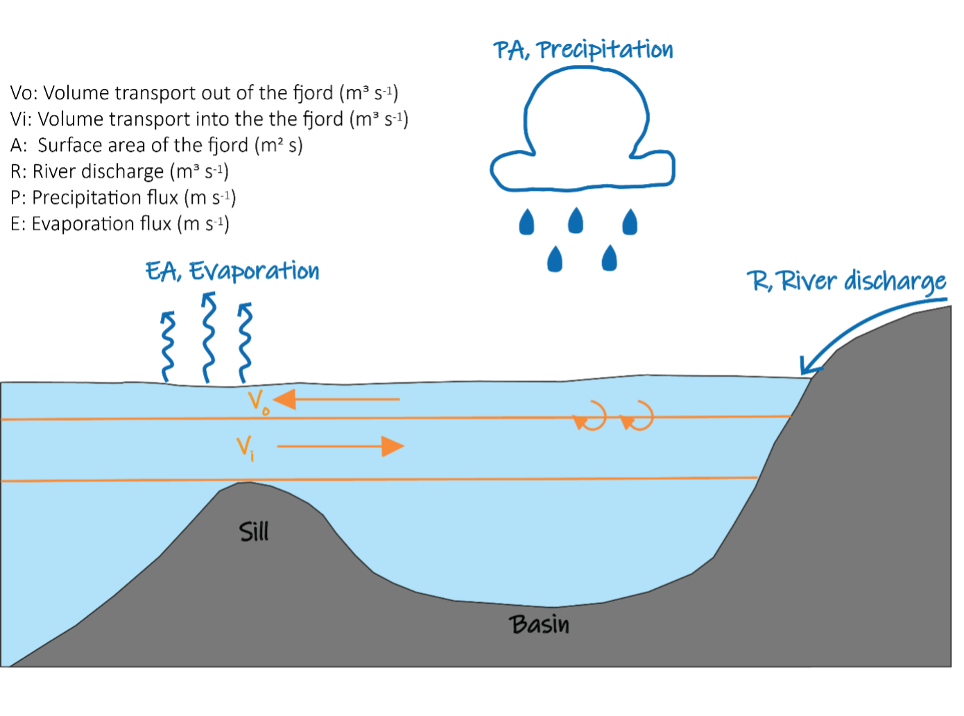
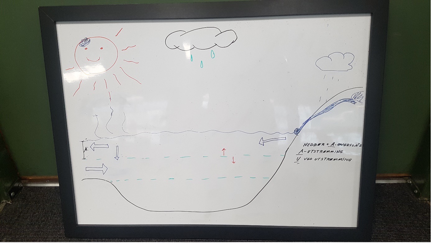
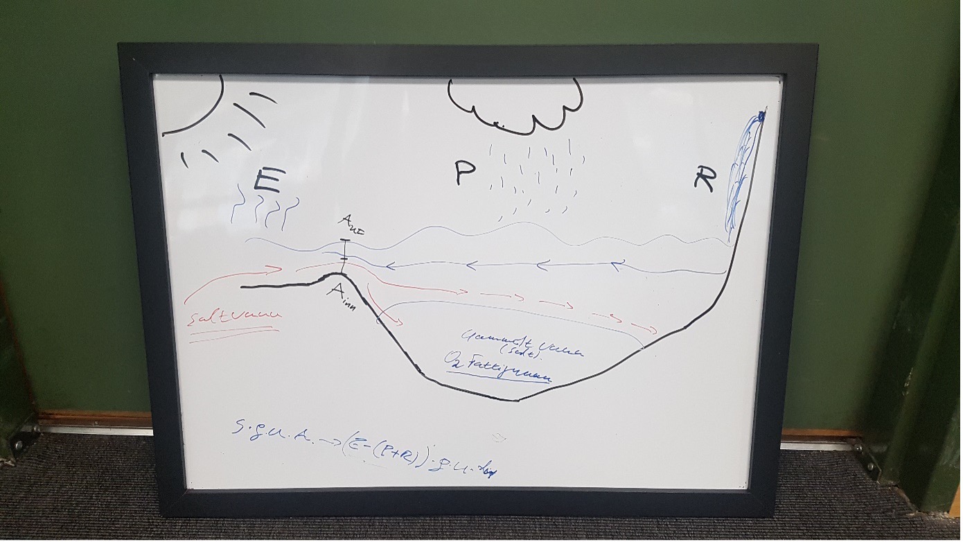
Example of sketch showing the fjord circulation with freshwater sinks/sources and flow scheme
Students often agree on a correct layering of the fjord, but struggle to determine flow directions. Instead of providing the solution, we give a mini-lecture on the conservation of volume and mass (salt), leading to Knudsen’s relations (Knudsen, 1900) for flow in a two-layer fjord.
Conservation of volume:
Volume in = Volume out
Vo +R + PA = Vo +EA,
- Vo-Vi =(R+PA)-EA =F, where F is the sum of the freshwater fluxes
Conservation of salt:
Salt inn = Salt out
ρiViSi = ρoVoSo
We simplify by disregarding the difference in ρi and ρo. Here, we typically calculate that there is a 3%
difference in density for ρo =1000 kg mᵌ and ρ1 =1030 kg mᵌ.
- ViSi = VoSo
Knudsen’s relations:
By combining equations (i-ii), we arrive at the Knudsen’s relations for volume transport in the the two layers above the sill:
Students can now use the conservation of volume idea to argue that there must be flow both into the fjord and out of the fjord. Using the Knudsen’s relations and assigning typical values for Si and So, students can look at the signs of Vo and Vi to arrive at the flow direction in each layer. This is also a great exercise to show students how we can strengthen an argument made by reasoning (because it makes the most sense) by a mathematical argument (test by applying established equations).
Applications
When the students have made conclusions about the sketches and the flow scheme (estuarine circulation), we can explore further the meaning of the Knudsen relations. We do this both with simple idealized examples and with numerical exercises based on real data from fjords.
For the idealized cases, we can provide students with depths and salinities of two layers, as well as a number for the freshwater flux. There are two main cases to study: -the fjord case (F>0), and the Mediterranean Sea case (F<0). The flow in these two examples is opposite, which causes interesting discussions among the students. They can compare the volume transports and discuss both direction and strength relative to the freshwater input.
To practice data analysis, students get ready-made python code, where, e.g., monthly river discharge and precipitation are available for further analysis. From hydrography profiles, the students can estimate the layer thicknesses and salinities, and calculate the volume transports and current velocities.
Examples of student sketches of the fjord circulation
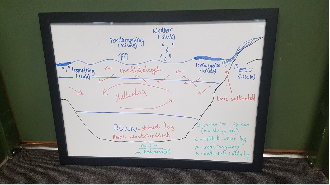
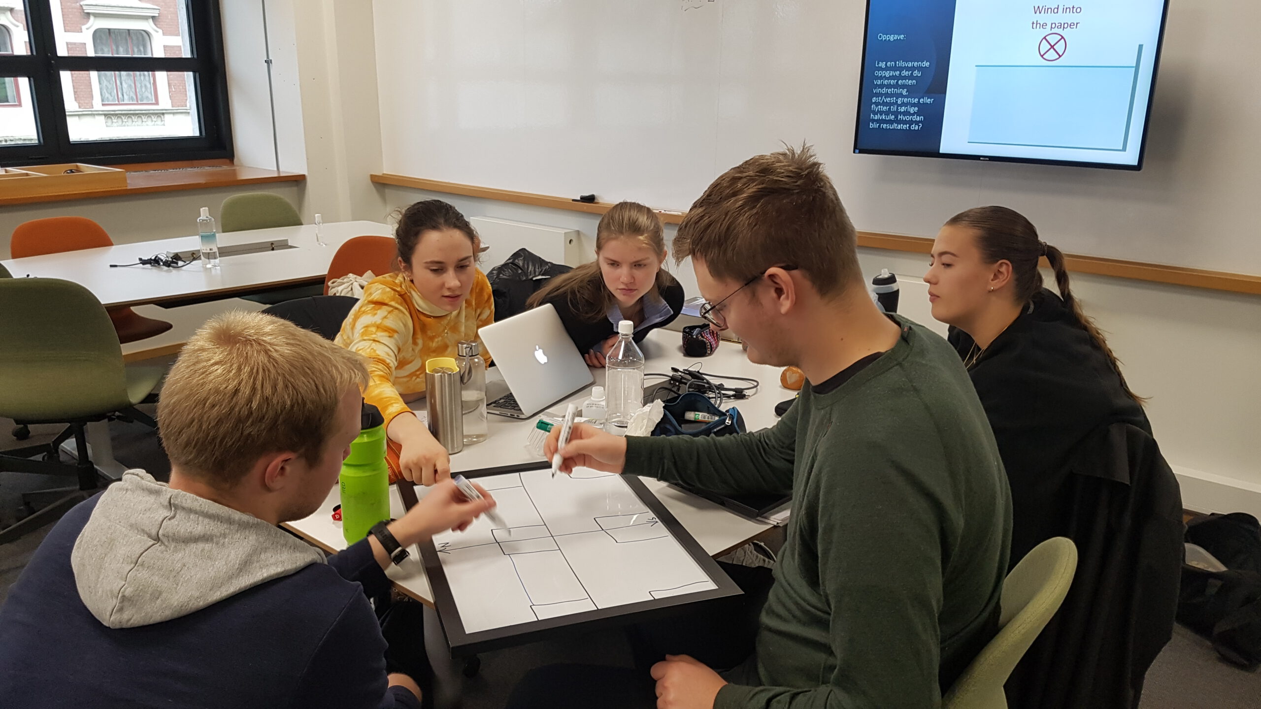
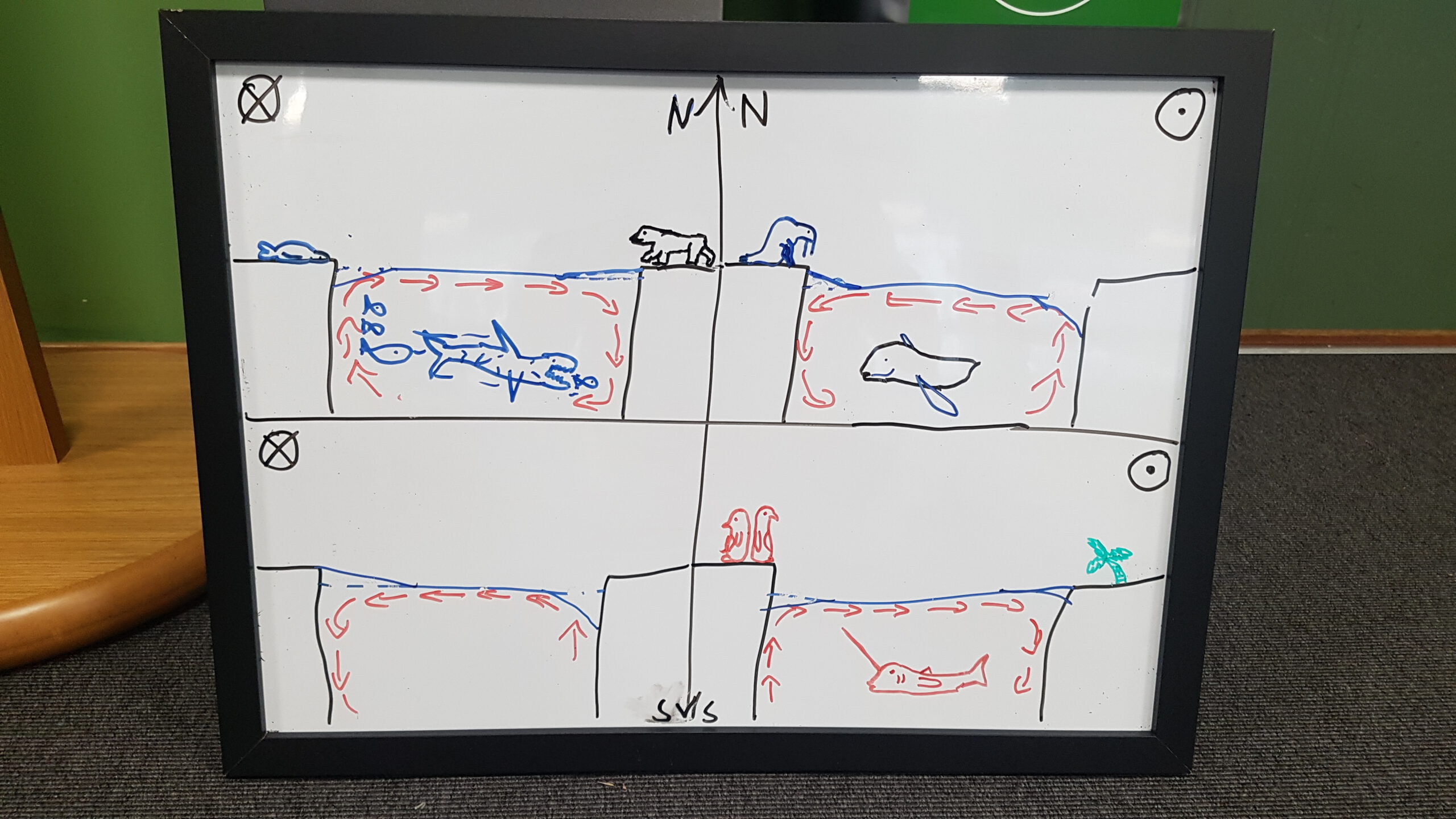
And this is what it looks like when students are working together on a similar task (on coastal up- and downwelling, see outcome of that below)
References
Daae, K., and M.S. Glessmer. 2022. Collaborative sketching to support sensemaking: If you can sketch it, you can explain it. Oceanography, https://doi.org/10.5670/oceanog.2022.208.
Knudsen, M. 1900. Ein hydrographischer Lehrsatz. Annalen der Hydrographie und Maritimen Meteorologie 28:316–320.