My friend Pierré and I started working on this article when both of us were still working at the Geophysical Institute in Bergen. It took forever to get published, mainly because both of us had moved on to different jobs with other foci, so maybe it’s not a big deal that it took me over a year to blog it? Anyway, I still think it is very important to introduce any kind of rotating experiments by first making sure people don’t harbour misconceptions about the Coriolis effect, and this is the best way we came up with to do so. But I am happy to hear any suggestions you might have on how to improve it :-)
Supporting Conceptual Understanding of the Coriolis Force Through Laboratory Experiments
By Dr. Mirjam S. Glessmer and Pierré D. de Wet
Published in Current: The Journal of Marine Education, Volume 31, No 2, Winter 2018
Do intriguing phenomena sometimes capture your attention to the extent that you haveto figure out why they work differently than you expected? What if you could get your students hooked on your topic in a similar way?
Wanting to comprehend a central phenomenon is how learning works best, whether you are a student in a laboratory course or a researcher going through the scientific process. However, this is not how introductory classes are commonly taught. At university, explanations are often presented or developed quickly with a focus on mathematical derivations and manipulations of equations. Room is seldom given to move from isolated knowledge to understanding where this knowledge fits in the bigger picture formed of prior knowledge and experiences. Therefore, after attending lectures and even laboratories, students are frequently able to give standard explanations and manipulate equations to solve problems, but lack conceptual understanding (Kirschner & Meester, 1988): Students might be able to answer questions on the laws of reflection, yet not understand how a mirror works, i.e. why it swaps left-right but not upside-down (Bertamini et al., 2003).
Laboratory courses are well suited to address and mitigate this disconnect between theoretical knowledge and practical application. However, to meet this goal, they need to be designed to focus specifically on conceptual understanding rather than other, equally important, learning outcomes, like scientific observation as a skill or arguing from evidence (NGSS, 2013), calculations of error propagations, application of specific techniques, or verifying existing knowledge, i.e. illustrating the lecture (Kirschner & Meester, 1988).
Based on experience and empirical evidence, students have difficulties with the concept of frames of reference, and especially with fictitious forces that are the result of using a different frame of reference. We here present how a standard experiment on the Coriolis force can support conceptual understanding, and discuss the function of employing individual design elements to maximize conceptual understanding.
HOW STUDENTS LEARN FROM LABORATORY EXPERIMENTS
In introductory-level college courses in most STEM disciplines, especially in physics-based ones like oceanography or meteorology and all marine sciences, laboratory courses featuring demonstrations and hands-on experiments are traditionally part of the curriculum.
Laboratory courses can serve many different and valuable learning outcomes: learning about the scientific process or understanding the nature of science, practicing experimental skills like observation, communicating about scientific content and arguing from evidence, and changing attitudes (e.g. Feisel & Rosa, 2005; NGSS, 2013; Kirschner & Meester, 1988; White, 1996). One learning outcome is often desired, yet for many years it is known that it is seldomly achieved: increasing conceptual understanding (Kirschner & Meester, 1988, Milner-Bolotin et al., 2007). Under general dispute is whether students actually learn from watching demonstrations and conducting lab experiments, and how learning can be best supported (Kirschner & Meester, 1988; Hart et al., 2000).
There are many reasons why students fail to learn from demonstrations (Roth et al., 1997). For example, in many cases separating the signal to be observed from the inevitably measured noise can be difficult, and inference from other demonstrations might hinder interpretation of a specific experiment. Sometimes students even “remember” witnessing outcomes of experiments that were not there (Milner-Bolotin et al., 2007). Even if students’ and instructors’ observations were the same, this does not guarantee congruent conceptual understanding and conceptual dissimilarity may persist unless specifically addressed. However, helping students overcome deeply rooted notions is not simply a matter of telling them which mistakes to avoid. Often, students are unaware of the discrepancy between the instructors’ words and their own thoughts, and hear statements by the instructor as confirmation of their own thoughts, even though they might in fact be conflicting (Milner-Bolotin et al., 2007).
Prior knowledge can sometimes stand in the way of understanding new scientific information when the framework in which the prior knowledge is organized does not seem to organically integrate the new knowledge (Vosniadou, 2013).The goal is, however, to integrate new knowledge with pre-existing conceptions, not build parallel structures that are activated in context of this class but dormant or inaccessible otherwise. Instruction is more successful when in addition to having students observe an experiment, they are also asked to predict the outcome before the experiment, and discuss their observations afterwards (Crouch et al., 2004). Similarly, Muller et al. (2007) find that even learning from watching science videos is improved if those videos present and discuss common misconceptions, rather than just presenting the material textbook-style. Dissatisfaction with existing conceptions and the awareness of a lack of an answer to a posed question are necessary for students to make major changes in their concepts (Kornell, 2009, Piaget, 1985; Posner et al., 1982). When instruction does not provide explanations that answer students’ problems of understanding the scientific point of view from the students’ perspective, it can lead to fragmentation and the formation of synthetic models (Vosniadou, 2013).
One operationalization of a teaching approach to support conceptual change is the elicit-confront-resolve approach (McDermott, 1991), which consists of three steps: Eliciting a lingering misconception by asking students to predict an experiment’s outcome and to explain their reasons for the prediction, confronting students with an unexpected observation which is conflicting with their prediction, and finally resolving the matter by having students come to a correct explanation of their observation.
HOW STUDENTS TRADITIONALLY LEARN ABOUT THE CORIOLIS FORCE
The Coriolis force is essential in explaining formation and behavior of ocean currents and weather systems we observe on Earth. It thus forms an important part of any instruction on oceanography, meteorology or climate sciences. When describing objects moving on the rotating Earth, the most commonly used frame of reference would be fixed on the Earth, so that the motion of the object is described relative to the rotating Earth. The moving object seems to be under the influence of a deflecting force – the Coriolis force – when viewed from the co-rotating reference frame. Even though the movement of an object is independent of the frame of reference (the set of coordinate axes relative to which the position and movement of an object is described is arbitrary and usually made such as to simplify the descriptive equations of the object), this is not immediately apparent.
Temporal and spatial frames of reference have been described as thresholds to student understanding (Baillie et al., 2012, James, 1966; Steinberg et al., 1990). Ever since its first mathematical description in 1835 (Coriolis, 1835), this concept is most often taught as a matter of coordinate transformation, rather than focusing on its physical relevance (Persson, 1998). Most contemporary introductory books on oceanography present the Coriolis force in that form (cf. e.g. Cushman-Roisin, 1994; Gill, 1982; Pinet, 2009; Pond and Pickard, 1983; Talley et al., 2001; Tomczak and Godfrey, 2003; Trujillo and Thurman, 2013). The Coriolis force is therefore often perceived as “a ‘mysterious’ force resulting from a series of ‘formal manipulations’” (Persson, 2010). Its unintuitive and seemingly un-physical character makes it difficult to integrate into existing knowledge and understanding, and “even for those with considerable sophistication in physical concepts, one’s first introduction to the consequences of the Coriolis force often produces something analogous to intellectual trauma” (Knauss, 1978).
In many courses, helping students gain a deeper understanding of rotating systems and especially the Coriolis force, is approached by presenting demonstrations, typically of a ball being thrown on a merry-go-round, showing the movement simultaneously from a rotating and a non-rotating frame (Urbano & Houghton, 2006), either in the form of movies or simulations, or in the lab as demonstration, or as a hands-on experiment[i]. After conventional instruction that exposed students to discussions and simulations, students are able to do calculations related to the Coriolis force.
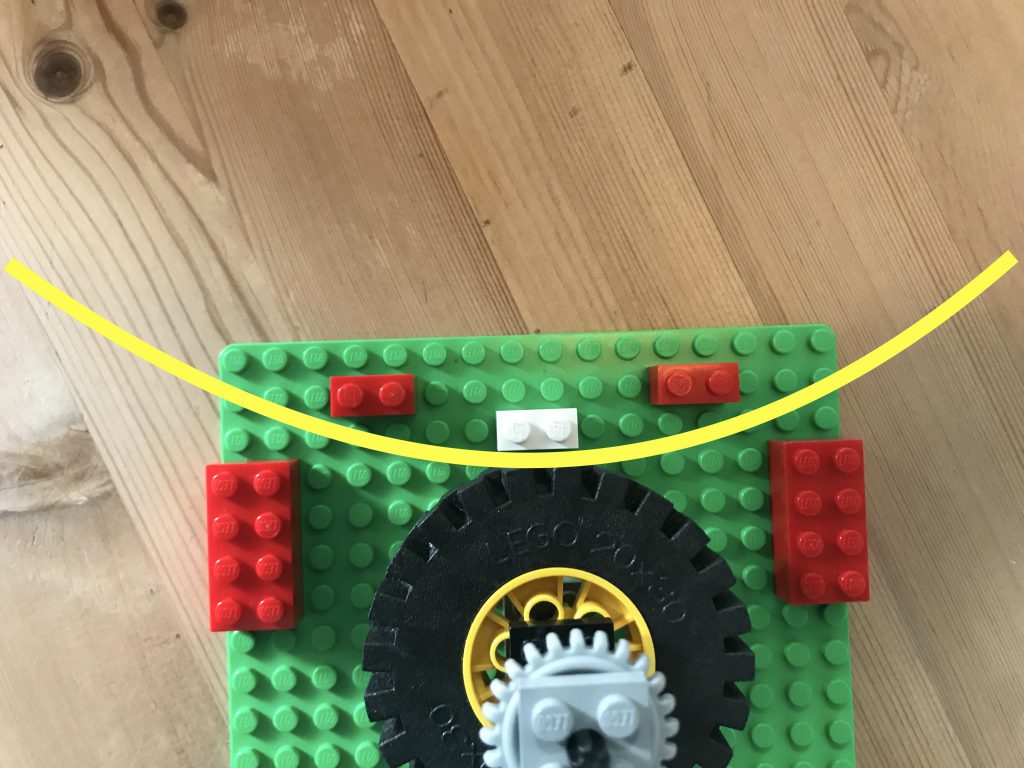
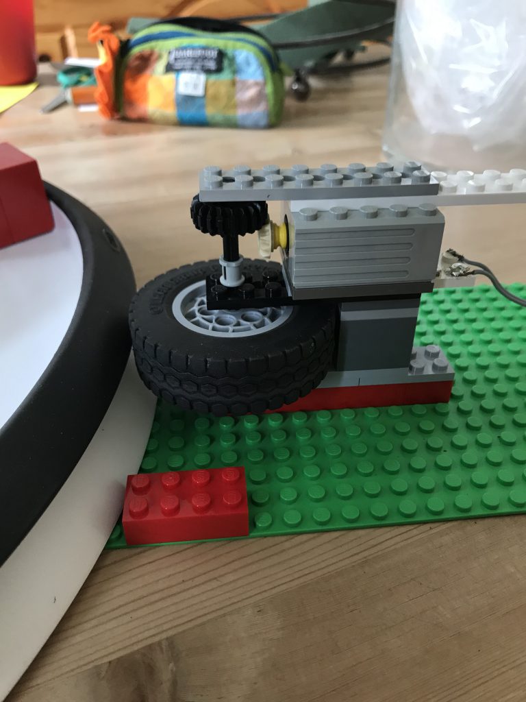
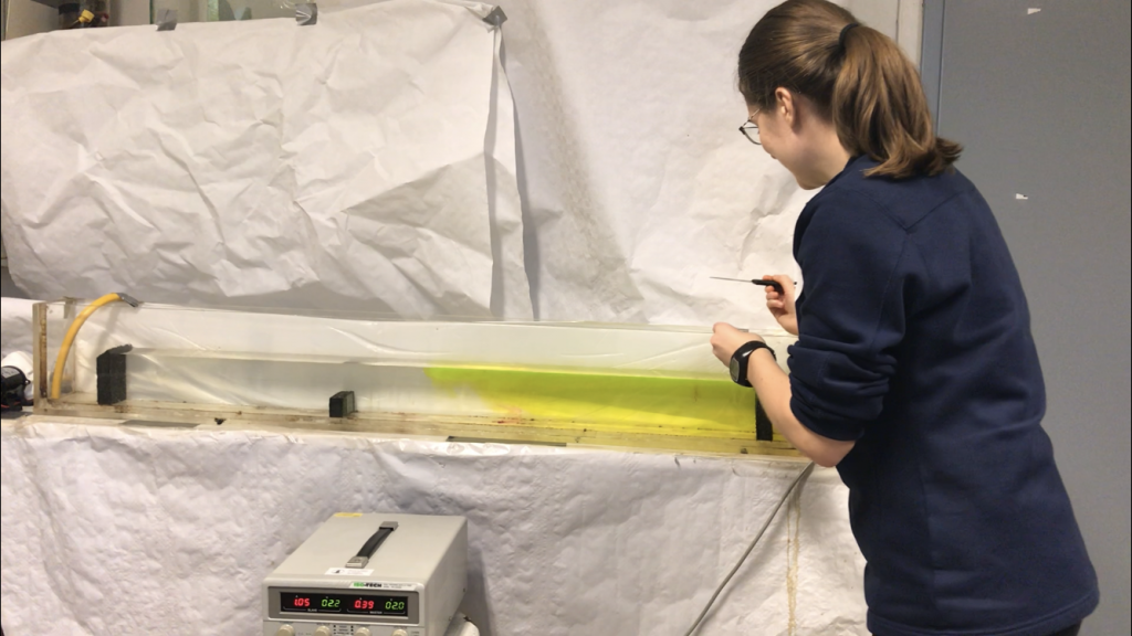
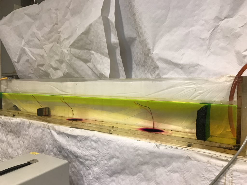
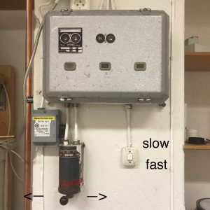
Nevertheless, when confronted with a real-life situation where they themselves are not part of the rotating system, students show difficulty in anticipating the movement of an object on a rotating body. In a traditional Coriolis experiment (Figure1), for example, a student launches a marble from a ramp on a rotating table (Figure 2A, B) and the motion of the marble is observed from two vantage points: where they are standing in the room, i.e. outside of the rotating system of the table; and on a screen that displays the table, as captured by a co-rotating camera mounted above it. When asked, before that experiment, what path the marble on the rotating surface will take, students report that they anticipate observing a deflection, its radius depending on the rotation’s direction and rate. After having observed the experiment, students report that they saw what they expected to see even though it never happened. Contextually triggered, knowledge elements are invalidly applied to seemingly similar circumstances and lead to incorrect conclusions (DiSessa & Sherin, 1988; Newcomer, 2010). This synthetic model of always expecting to see a deflection of an object moving on a rotating body, no matter which system of reference it is observed from, needs to be modified for students to productively work with the concept of the Coriolis force.
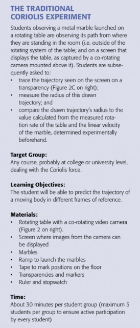
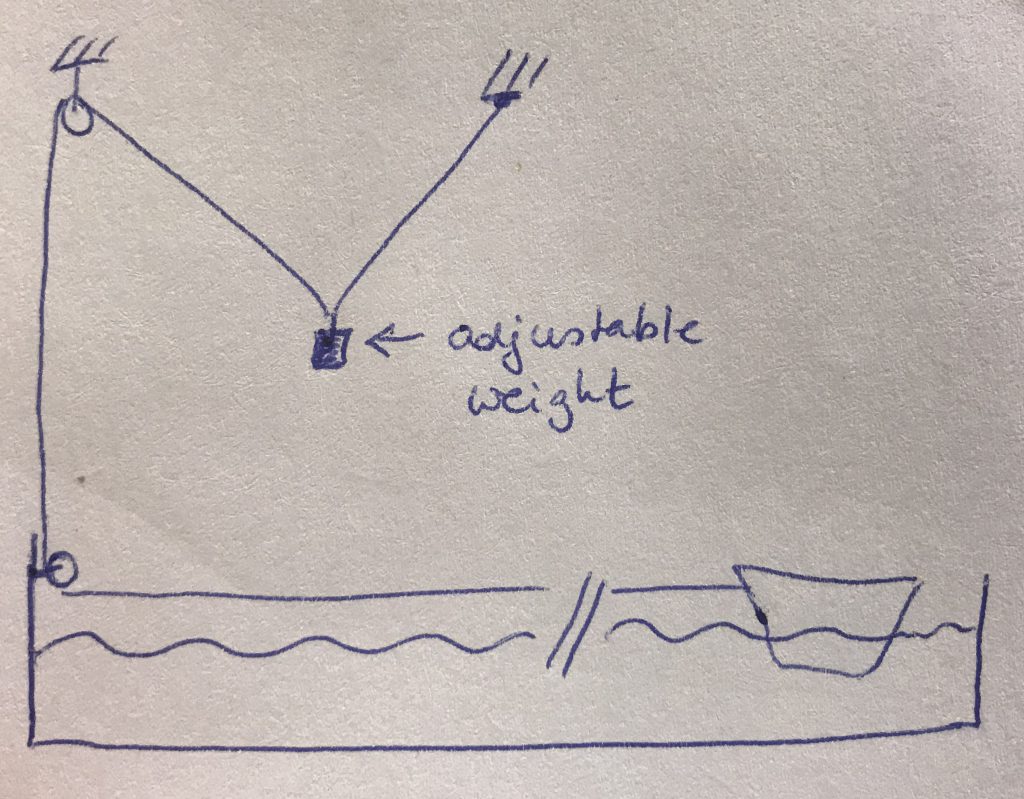
Figure 1: Details of the Coriolis experiment
Despite these difficulties in interpreting the observations and understanding the underlying concepts, rotating tables recently experienced a rise in popularity in undergraduate oceanography instruction (Mackin et al., 2012) as well as outreach to illustrate features of the oceanic and atmospheric circulation(see for example Marshall and Plumb, 2007). This makes it even more important to consider what students are intended to learn from such demonstrations or experiments, and how these learning outcomes can be achieved.
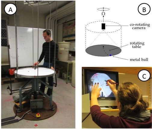
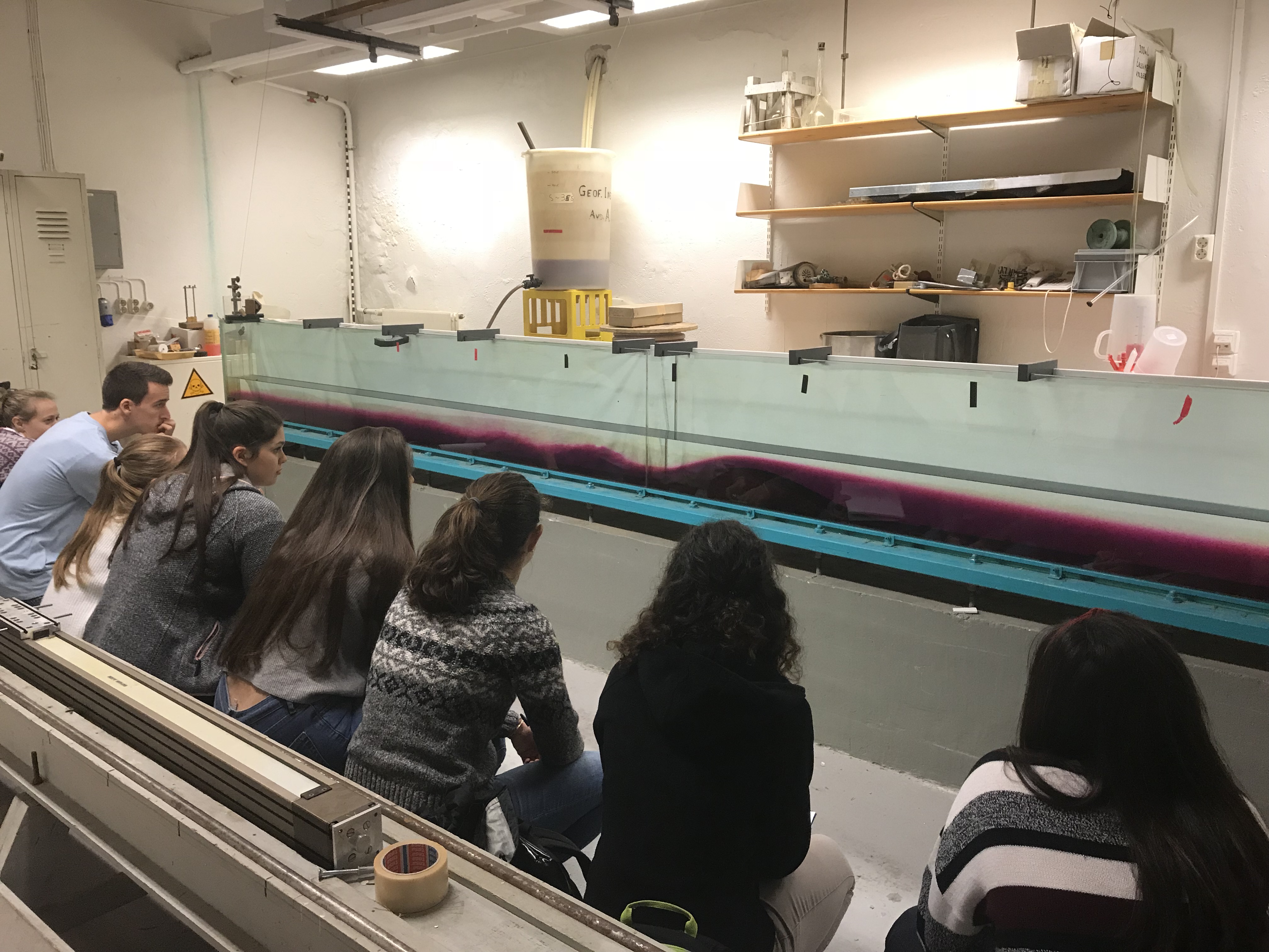
Figure 2A: View of the rotating table including the video camera on the scaffolding above the table. B: Sketch of the rotating table, the mounted (co-rotating) camera, and the marble on the table. C: Student tracing the curved trajectory of the marble on a transparency. On the screen, the experiment is shown as captured by the co-rotating camera, hence in the rotating frame of reference.
A RE-DESIGNED HANDS-ON INTRODUCTION TO THE CORIOLIS FORCE
The traditional Coriolis experiment, featuring a body on a rotating table[ii], observed both from within and from outside the rotating system, can be easily modified to support conceptual understanding.
When students of oceanography are asked to do a “dry” experiment (in contrast to a “wet” one with water in a tank on the rotating table) on the Coriolis force, at first, this does not seem like a particularly interesting phenomenon to students because they believe they know all about it from the lecture already. The experiment quickly becomes intriguing when a cognitive dissonance arises and students’ expectations do not match their observations. We use an elicit-confront-resolve approach to help students observe and understand the seemingly conflicting observations made from inside versus outside of the rotating system (Figure 3). To aid in making sense of their observations in a way that leads to conceptual understanding the three steps elicit, confront, and resolve are described in detail below.

Figure 3: Positions of the ramp and the marble as observed from above in the non-rotating (top) and rotating (bottom) case. Time progresses from left to right. In the top plots, the positions are shown in inert space. From left to right, the current positions of the ramp and marble are added with gradually darkening colors. In the bottom plots, the ramp stays in the same position relative to the co-rotating observer, but the marble moves and the current position is always displayed with the darkest color.
2. What do you think will happen? Eliciting a (possibly) lingering misconception
Students have been taught in introductory lectures that any moving object in a counter-clockwise rotating system (i.e. in the Northern Hemisphere) will be deflected to the right. They are also aware that the extent to which the object is deflected depends on its velocity and the rotational speed of the reference frame. In our experience, due to this prior schooling, students expect to see a Coriolis deflection even when they observe a rotating system “from the outside”. When the conventional experiment is run without going through the additional steps described here, students often report having observed the (non-existent) deflection.
By activating this prior knowledge and discussing what students anticipate observing under different conditions before the actual experiment is conducted, the students’ insights are put to the test. This step is important since the goal is to integrate new knowledge with pre-existing conceptions, not build parallel structures that are activated in context of this class but dormant or inaccessible otherwise. Sketching different scenarios (Fan, 2015; Ainsworth et al., 2011) and trying to answer questions before observing experiments support the learning process since students are usually unaware of their premises and assumptions (Crouch et al., 2004). Those need to be explicated and documented (even just by saying them out loud) before they can be tested, and either be built on, or, if necessary, overcome.
We therefore ask students to observe and describe the path of a marble being radially launched from the perimeter of the circular, non-rotating table by a student standing at a marked position next to the table, the “launch position”. The marble is observed rolling towards and over the center point of the table, dropping off the table diametrically opposite from the position from which it was launched. So far nothing surprising. A second student – the catcher– is asked to stand at the position where the marble dropped off the table’s edge so as to catch the marble in the non-rotating case. The position is also marked on the floor with tape to document the observation.
Next, the experimental conditions of this thought experiment (Winter, 2015) are varied to reflect on how the result depends on them. The students are asked to predict the behavior of the marble once the table is put into slow rotation. At this point, students typically enquire about the direction of rotation and, when assured that “Northern Hemisphere” counter-clockwise rotation is being applied, their default prediction is that the marble will be deflected to the right. When asked whether the catcher should alter their position, the students commonly answer that the catcher should move some arbitrary angle, but typically less than 90 degrees, clockwise around the table. The question of the influence of an increase in the rotational rate of the table on the catcher’s placement is now posed. “Still further clockwise”, is the usual answer. This then leads to the instructor’s asking whether a rotational speed exists at which the student launching the marble, will also be able to catch it themselves. Usually the students confirm that such a situation is indeed possible.
2. Did you observe what you expected to see? Confronting the misconception
After “eliciting” student conceptions, the “confront” step serves to show the students the discrepancy between what they expect to see, and what they actually observe. Starting with the simple, non-rotating case, the marble is launched again and the nominated catcher, positioned diametrically across from the launch position, seizes the marble as it falls off the table’s surface right in front of them. As theoretically discussed beforehand, the table is then put into rotation at incrementally increasing rates, with the marble being launched from the same position for each of the different rotational speeds. It becomes clear that the catcher can – without any adjustments to their position – remain standing diametrically opposite to the student launching the marble – the point where the marble drops to the floor. Hence students realize that the movement of the marble relative to the non-rotating laboratory is unaffected by the table’s rotation rate.
This observation appears counterintuitive, since the camera, rotating with the system, shows the curved trajectories the students had expected; segments of circles with decreasing radii as the rotation rate increases. Furthermore, to add to the confusion, when observed from their positions around the rotating table, the path of the marble on the rotating table appears to show a deflection, too. This is due to the observer’s eye being fooled by focusing on features of the table, e.g. marks on the table’s surface or the bars of the camera scaffold, relative to which the marble does, indeed, follow a curved trajectory. To overcome this optical illusion, the instructor may ask the students to crouch, diametrically across from the launcher, so that their line of sight is aligned with the table’s surface, i.e. at a zero-zenith angle of observation. From this vantage point, the marble is observed to indeed be moving in a straight line towards the observer, irrespective of the rotation rate of the table. Observing from different perspectives and with focus on different aspects (Is the marble coming directly towards me? Does it fall on the same spot as before? Did I need to alter my position in the room at all?) helps students gain confidence in their observations.
To solidify the concept, the table may again be set into rotation. The launcher and the catcher are now asked to pass the marble to one another by throwing it across the table without it physically making contact with the table’s surface. As expected, the marble moves in a straight line between the launcher and the catcher, whom are both observing from an inert frame of reference. However, when viewing the playback of the co-rotating camera, which represents the view from the rotating frame of reference, the trajectory is observed as curved[iii].
3. Do you understand what is going on? Resolving the misconception
Misconceptions that were brought to light during the “elicit” step, and whose discrepancy with observations was made clear during the “confront” step, are finally resolved in this step. While this sounds very easy, in practice it is anything but. For learning to take place, the instructor needs to aid students in reflecting upon and reassessing previous knowledge by pointing out and dispelling any remaining implicit assumptions, making it clear that the discrepant trajectories are undoubtedly the product of viewing the motion from different frames of reference. Despite the students’ observations and their participation in the experiment this does not happen instantaneously. Oftentimes further, detailed discussion is required. Frequently students have to re-run the experiment themselves in different roles (i.e. as launcheras well as catcher) and explicitly state what they are noticing before they trust their observations.
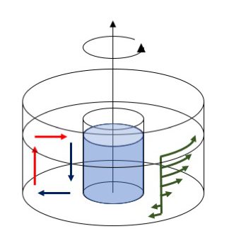
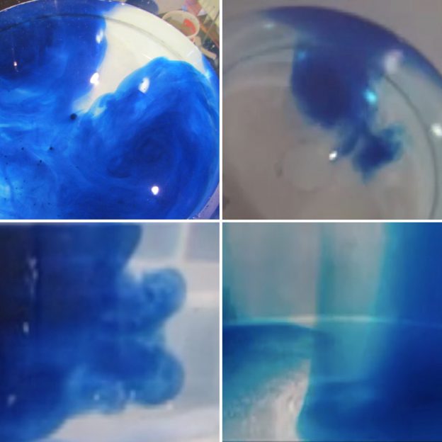
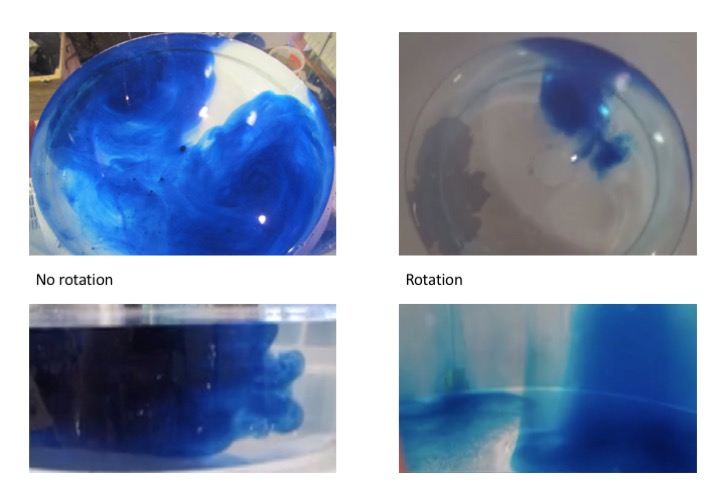
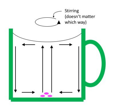
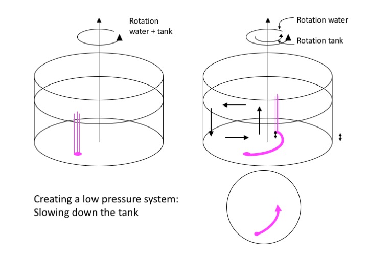
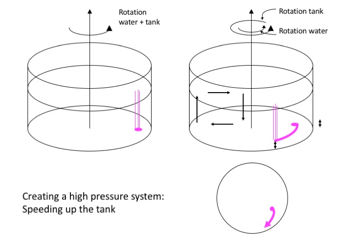
For this experiment to benefit the learning outcomes of the course, which go beyond understanding of a marble on a rotating table and deal with ocean and atmosphere dynamics, knowledge needs to be integrated into previous knowledge structures and transferred to other situations. This could happen by discussion of questions like, for example: How could the experiment be modified such that a straight trajectory is observed on the screen? What would we expect to observe if we added a round tank filled with water and paper bits floating on it to the table and started rotating it? How are our observations of these systems relevant and transferable to the real world? What are the boundaries of the experiment?
IS IT WORTH THE EXTRA EFFORT? DISCUSSION
We taught an undergraduate laboratory course which included this experiment for several years. In the first year, we realized that the conventional approach was not effective. In the second year, we tried different instructional approaches and settled on the one presented here. We administered identical work sheets before and after the experiment. These work sheets were developed as instructional materials to ensure that every student individually went through the elicit-confront-resolve process. Answers on those worksheets show that all our students did indeed expect to see a deflection despite observing from an inert frame of reference: Students were instructed to consider both a stationary table and a table rotating at two different rates. They were then asked to, for each of the scenarios, mark with an X the location where they thought the marble would contact the floor after dropping off the table’s surface. Before instruction, all students predicted that the marble would hit the floor in different spots – diametrically across from the launch point for no rotation, and at increasing distances from that first point with increasing rotation rates of the table (Figure 4). This is the exact misconception we aimed to elicit with this question: students were applying correct knowledge (“in the Northern Hemisphere a moving body will be deflected to the right”) to situations where this knowledge was not applicable: when observing the rotating body and the moving object upon it from an inert frame of reference.
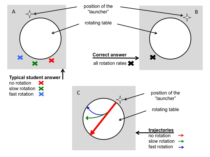
Figure 4A: Depiction of the typical wrong answer to the question: Where would a marble land on the floor after rolling across a table rotating at different rotation rates? B: Correct answer to the same question. C: Correct traces of marbles rolling across a rotating table.
In a second question, students were asked to imagine the marble leaving a dye mark on the table as it rolls across it, and to draw these traces left on the table. In this second question, students were thus required to infer that this would be analogous to regarding the motion of the marble as observed from the co-rotating frame of reference. Drawing this trajectory correctly before the experiment is run does not imply a correct conceptual understanding, since the transfer between rotating and non-rotating frames of references is not happening yet and students draw curved trajectories for all cases. However, after the experiment this question is useful especially in combination with the first one, as it requires a different answer than the first, and an answer that students just learned they should not default to.
The students’ laboratory reports supply additional support of the usefulness of this new approach. These reports had to be submitted a week after doing the experiment and accompanying work sheets, which were collected by the instructors. One of the prompts in the lab report explicitly addresses observing the motion from an inert frame of reference as well as the influence of the table’s rotational period on such motion. This question was answered correctly by all students. This is remarkable for three reasons: firstly, because in the previous year with conventional instruction, this question was answered incorrectly by the vast majority of students; secondly, from our experience, lab reports have a tendency to be eerily similar year after year which did not hold true for tis specific question; and lastly, because for this cohort, it is one of very few questions that all students answered correctly in their lab reports, which included seven experiments in addition to the Coriolis experiment. These observations lead us to believe that students do indeed harbor the misconception we suspected, and that the modified instructional approach has supported conceptual change.
CONCLUSIONS
We present modifications to a “very simple” experiment and suggest running it before subjecting students to more advanced experiments that illustrate concepts like Taylor columns or weather systems. These more complex processes and experiments cannot be fully understood without first understanding the Coriolis force acting on the arguably simplest bodies. Supplying correct answers to standard questions alone, e.g. “deflection to the right on the northern hemisphere”, is not sufficient proof of understanding.
In the suggested instructional strategy, students are required to explicitly state their expectations about what the outcome of an experiment will be, even though their presuppositions are likely to be wrong. The verbalizing of their assumptions aids in making them aware of what they implicitly hold to be true. This is a prerequisite for further discussion and enables confrontation and resolution of potential misconceptions. Wesuggest using an elicit-confront-resolve approach even when the demonstration is not run on an actual rotating table, but virtually conducted instead, for example using Urbano & Houghton (2006)’s Coriolis force simulation. We claim that the approach is nevertheless beneficial to increasing conceptual understanding.
We would like to point out that gaining insight from any seemingly simple experiment, such as the one discussed in this article, might not be nearly as straightforward or obvious for the students as anticipated by the instructor. Using an intriguing phenomenon to be investigated experimentally, and slightly changing conditions to understand their influence on the result, is highly beneficial. Probing for conceptual understanding in new contexts, rather than the ability to calculate a correct answer, proved critical in understanding where the difficulties stemmed from, and only a detailed discussion with several students could reveal the scope of difficulties.
ACKNOWLEDGEMENTS
The authors are grateful for the students’ consent to be featured in this article’s figures.
RESOURCES
Movies of the experiment can be seen here:
Rotating case: https://vimeo.com/59891323
Non-rotating case: https://vimeo.com/59891020
Using an old disk player and a ruler in absence of a co-rotating camera: https://vimeo.com/104169112
REFERENCES
Ainsworth, S., Prain, V., & Tytler, R. 2011. Drawing to Learn in Science Science, 333(6046), 1096-1097 DOI: 10.1126/science.1204153
Baillie, C., MacNish, C., Tavner, A., Trevelyan, J., Royle, G., Hesterman, D., Leggoe, J., Guzzomi, A., Oldham, C., Hardin, M., Henry, J., Scott, N., and Doherty, J.2012. Engineering Thresholds: an approach to curriculum renewal. Integrated Engineering Foundation Threshold Concept Inventory 2012. The University of Western Australia, <http://www.ecm.uwa.edu.au/__data/assets/pdf_file/0018/2161107/Foundation-Engineering-Threshold-Concept-Inventory-120807.pdf>
Bertamini, M., Spooner, A., & Hecht, H. (2003). Naïve optics: Predicting and perceiving reflections in mirrors. JOURNAL OF EXPERIMENTAL PSYCHOLOGY HUMAN PERCEPTION AND PERFORMANCE, 29(5), 982-1002.
Coriolis, G. G. 1835. Sur les équations du mouvement relatif des systèmes de corps. J. de l’Ecole royale polytechnique15: 144–154.
Crouch, C. H., Fagen, A. P., Callan, J. P., and Mazur. E. 2004. Classroom Demonstrations: Learning Tools Or Entertainment?. American Journal of Physics, Volume 72, Issue 6, 835-838.
Cushman-Roisin, B. 1994. Introduction to Geophysical Fluid DynamicsPrentice-Hall. Englewood Cliffs, NJ, 7632.
diSessa, A.A. and Sherin, B.L., 1998. What changes in conceptual change?. International journal of science education, 20(10), pp.1155-1191.
Durran, D. R. and Domonkos, S. K. 1996. An apparatus for demonstrating the inertial oscillation, BAMS, Vol 77, No 3
Fan, J. (2015). Drawing to learn: How producing graphical representations enhances scientific thinking. Translational Issues in Psychological Science, 1(2), 170-181 DOI: 10.1037/tps0000037
Gill, A. E. 1982. Atmosphere-ocean dynamics(Vol. 30). Academic Pr.
James, E.L., 1966. Acceleration= v2/r. Physics Education, 1(3), p.204.
Kornell, N., Jensen Hays, M., and Bjork, R.A. (2009), Unsuccessful Retrieval Attempts Enhance Subsequent Learning, Journal of Experimental Psychology: Learning, Memory, and Cognition 2009, Vol. 35, No. 4, 989–998
Hart, C., Mulhall, P., Berry, A., Loughran, J., and Gunstone, R. 2000.What is the purpose of this experiment? Or can students learn something from doing experiments?,Journal of Research in Science Teaching, 37(7), p 655–675
Kirschner, P.A. and Meester, M.A.M., 1988. The laboratory in higher science education: Problems, premises and objectives. Higher education, 17(1), pp.81-98.
Knauss, J. A. 1978. Introduction to physical oceanography. Englewood Cliffs, N.J: Prentice-Hall.
Mackin, K.J., Cook-Smith, N., Illari, L., Marshall, J., and Sadler, P. 2012. The Effectiveness of Rotating Tank Experiments in Teaching Undergraduate Courses in Atmospheres, Oceans, and Climate Sciences, Journal of Geoscience Education, 67–82
Marshall, J. and Plumb, R.A. 2007. Atmosphere, Ocean and Climate Dynamics, 1stEdition, Academic Press
McDermott, L. C. 1991. Millikan Lecture 1990: What we teach and what is learned – closing the gap, Am. J. Phys. 59 (4)
Milner-Bolotin, M., Kotlicki A., Rieger G. 2007. Can students learn from lecture demonstrations? The role and place of Interactive Lecture Experiments in large introductory science courses.The Journal of College Science Teaching, Jan-Feb, p.45-49.
Muller, D.A., Bewes, J., Sharma, M.D. and Reimann P. 2007.Saying the wrong thing: improving learning with multimedia by including misconceptions, Journal of Computer Assisted Learning (2008), 24, 144–155
Newcomer, J.L. 2010. Inconsistencies in Students’ Approaches to Solving Problems in Engineering Statics, 40th ASEE/IEEE Frontiers in Education Conference, October 27-30, 2010, Washington, DC
NGSS Lead States. 2013. Next generation science standards: For states, by states. National Academies Press.
Persson, A. 1998.How do we understand the Coriolis force?, BAMS, Vol 79, No 7
Persson, A. 2010.Mathematics versus common sense: the problem of how to communicate dynamic meteorology, Meteorol. Appl. 17: 236–242
Piaget, J. (1985). The equilibration of cognitive structure. Chicago: University of Chicago Press.
Pinet, P. R. 2009. Invitation to oceanography. Jones & Bartlett Learning.
Posner, G.J., Strike, K.A., Hewson, P.W. and Gertzog, W.A. 1982. Accommodation of a Scientific Conception: Toward a Theory of Conceptual Change. Science Education 66(2); 211-227
Pond, S. and G. L. Pickard 1983. Introductory dynamical oceanography. Gulf Professional Publishing.
Roth, W.-M., McRobbie, C.J., Lucas, K.B., and Boutonné, S. 1997. Why May Students Fail to Learn from Demonstrations? A Social Practice Perspective on Learning in Physics. Journal of Research in Science Teaching, 34(5), page 509–533
Steinberg, M.S., Brown, D.E. and Clement, J., 1990. Genius is not immune to persistent misconceptions: conceptual difficulties impeding Isaac Newton and contemporary physics students. International Journal of Science Education, 12(3), pp.265-273.
Talley, L. D., G. L. Pickard, W. J. Emery and J. H. Swift 2011. Descriptive physical oceanography: An introduction. Academic Press.
Tomczak, M., and Godfrey, J. S. 2003. Regional oceanography: an introduction. Daya Books.
Trujillo, A. P., and Thurman, H. V. 2013. Essentials of Oceanography, Prentice Hall; 11 edition (January 14, 2013)
Urbano, L.D., Houghton J.L., 2006. An interactive computer model for Coriolis demonstrations.Journal of Geoscience Education 54(1): 54-60
Vosniadou, S. (2013). Conceptual change in learning and instruction: The framework theory approach. International handbook of research on conceptual change, 2, 11-30.
White, R. T. 1996. The link between the laboratory and learning. International Journal of Science Education, 18(7), 761-774.
Winter, A., 2015. Gedankenexperimente zur Auseinandersetzung mit Theorie. In: Die Spannung steigern – Laborpraktika didaktisch gestalten.Schriften zur Didaktik in den IngenieurswissenschaftenNr. 3, M. S. Glessmer, S. Knutzen, P. Salden (Eds.), Hamburg
Endnotes
[i]While tremendously helpful in visualizing an otherwise abstract phenomenon, using a common rotating table introduces difficulties when comparing the observed motion to the motion on Earth. This is, among other factors, due to the table’s flat surface (Durran and Domonkos, 1996), the alignment of the (also fictitious) centrifugal force with the direction of movement of the marble (Persson, 2010), and the fact that a component of axial rotation is introduced to the moving object when launched. Hence, the Coriolis force is not isolated. Regardless of the drawbacks associated with the use of a (flat) rotating table to illustrate the Coriolis effect, we see value in using it to make the concept of fictitious forces more intuitive, and it is widely used to this effect.
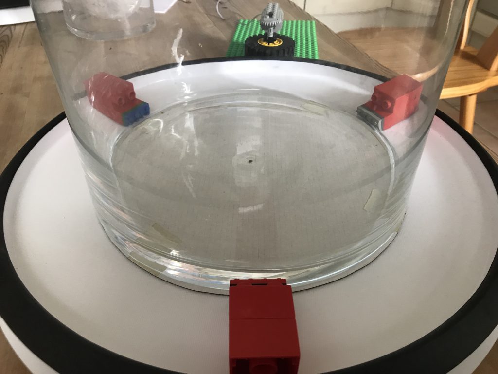
[ii]Despite their popularity in geophysical fluid dynamics instruction at many institutions, rotating tables might not be readily available everywhere. Good instructions for building a rotating table can, for example, be found on the “weather in a tank” website, where there is also the contact information to a supplier given: http://paoc.mit.edu/labguide/apparatus.html. A less expensive setup can be created from old disk players or even Lazy Susans, or found on playgrounds in form of merry-go-rounds. In many cases, setting the exact rotation rate is not as important as having a qualitative difference between “slow” and “fast” rotation, which is very easy to realize. In cases where a co-rotating camera is not available, by dipping the marble in either dye or chalk dust (or by simply running a pen in a straight line across the rotating surface), the trajectory in the rotating system can be visualized. The instructional approach described in this manuscript is easily adapted to such a setup.
[iii]We initially considered starting the lab session by throwing the marble diametrically across the rotating table. Students would then see on-screen the curved trajectory of a marble, which had never made physical contact with the table rotating beneath it, and which was clearly moving in a straight line from thrower to catcher, leading to the realization that it is the frame of reference that is to blame for the marble’s curved trajectory. However, the speed of a flying marble makes it very difficult to observe its curved path on the screen in real time. Replaying the footage in slow motion helps in this regard. Yet, replacing direct observation with recording and playback seemingly hampers acceptance of the occurrence as “real”. We therefore decided to only use this method to further illustrate the concept, not as a first step.
Bios
Dr. Mirjam Sophia Glessmer, holds a Master of Higher Education and Ph.D. in physical oceanography. She works at the Leibniz Institute of Science and Mathematics Education in Kiel, Germany. Her research focus lies on informal learning and science communication in ocean and climate sciences.
Pierre de Wet is a Ph.D. student in Oceanography and Climatology at the University of Bergen, Norway, and holds a Master in Applied Mathematics from the University of Stellenbosch, South Africa. He is employed by Akvasafe AS, where he works with the analysis and modelling of physical environmental parameters used in the mooring analysis and accreditation of floating fish farms.