Mirjam S. Glessmer & Pierré D. de Wet

Abstract

Even though experiments – whether demonstrated to, or personally performed by students – have been part of training in STEM for a long time, their effectiveness as an educational tool are sometimes questioned. For, despite students’ ability to produce correct answers to standard questions regarding these laboratory exercises, probing deeper often reveals a lack of conceptual understanding.

One way to help students make sense of experiments is to use them in combination with an elicit-confront-resolve approach. With this approach, before the experiment demonstrating a specific concept is run, students are asked to discuss the expected outcome in groups. In so doing, should (specific) misconceptions be harbored about the underlying concept, these are elicited. Incorrect student feedback (feedback illustrating that a misconception is present) is not corrected at this stage. As the demonstration plays out, a mismatch between observation and hypothesis confronts students with their misconceptions. Finally, repetition of the experiment and peer discussion as well as discussion with the instructor lead to resolving of the misunderstandings.

Here, we apply the elicit-confront-resolve approach to a standard demonstration in introductory dynamics, namely the interplay of a rotating frame of reference, movement of particles observed from outside that frame of reference and the resulting fictitious forces. The efficacy of the elicit-confront-resolve approach for this purpose is discussed. Additionally, recommendations are given on how to modify instruction to further aid students in interpreting and understanding their observations.

Key words

Coordinate system, frame of reference, fictitious force, hands-on experiment, elicit-confront-resolve

Introduction

In many STEM disciplines, demonstrations and hands-on experimentation have been part of the curriculum for a long time. However, whether students actually learn from watching demonstrations and conducting lab experiments, and how their learning can be best supported by the instructor, is under dispute (Hart et al, 2000). There are many reasons why students might fail to learn from demonstrations (Roth et al, 1997). For example, separating the signal to be observed from the inevitable noise can be difficult, and inference from other demonstrations might hinder interpretation of a specific experiment. Sometimes students even “remember” witnessing outcomes of experiments that were not there (Milner-Bolotin, Kotlicki, and Rieger (2007)).

Even if students’ and instructors’ observations were the same, this does not guarantee congruent conceptual understanding and conceptual dissimilarity may persist unless specifically treated. However, helping students overcome deeply rooted notions is not simply a matter of telling them which mistakes to avoid. Often they are unaware of the discrepancy between the instructors’ words and their own thoughts (Milner-Bolotin, Kotlicki, and Rieger (2007)).

One way to address misconceptions is by using an elicit-confront-resolve approach (McDermott, 1991). Posner et al. (1982) suggested that dissatisfaction with existing conceptions, which in this method is purposefully created in the confront-step, is necessary for students to make major changes in their concepts. As shown by Kornell (2009), this approach enhances learning by confronting the student with their lack of an answer to a posed question. Similarly, Muller et al. (2007) find that learning from watching science videos is improved if those videos present and discuss common misconceptions, rather than just presenting material textbook-style.

In this article we look at how an elicit-confront-resolve approach can further student engagement and learning. This is done by using a typical introductory demonstration in geophysical fluid dynamics, namely the effect of rotation on the movement of a ball as seen from within and from outside the rotating system. The motivation for the choice of experiment is dual: the rising popularity of rotating tables in undergraduate oceanography instruction (Mackin et al, 2012), and the difficulties students display in anticipating the movement of an object on a rotating body when they themselves are not part of the rotating system.

The Coriolis force as example for the instructional method

On a rotating earth, all large-scale motion is subject to the influence of the fictitious Coriolis force, and without a solid understanding of the Coriolis force it is impossible to understand the movement of ocean currents or weather systems. Furthermore, the Coriolis force forms an important part of classical oceanographic theories, such as the Ekman spiral, inertial oscillations, topographic steering and geostrophic currents. A thorough understanding of the concept of fictitious forces and observations in rotating vs. non-rotating systems is thus essential in order to gain a deeper understanding of these systems. Therefore, most introductory books on oceanography, or more generally geophysical fluid dynamics, present the concept in some form or other (cf. e.g. Cushman-Roisin (1994), Gill (1982), Pinet (2009), Pond and Pickard (1983), Talley et al. (2001), Tomczak and Godfrey (2003), Trujillo and Thurman (2013)). Yet, temporal and spatial frames of reference have been described as thresholds to student understanding (Baillie et al., 2012).

The frame of reference is the chosen set of coordinate axes relative to which the position and movement of an object is described. The choice of axes is arbitrary and usually made such as to simplify the descriptive equations of the object under regard. Any object can thus be described in relation to different frames of reference. When describing objects moving on the rotating Earth, the most commonly used frame of reference would be fixed on the Earth (co-rotating), so that the motion of the object is described relative to the rotating Earth. Alternatively, the motion of the same object could be described in an inert frame of reference outside of the rotating Earth. Even though the movement of the object is independent of the frame of reference used to describe it, this independence is not immediately apparent. Objects moving on the rotating Earth seemingly experience a deflecting force when viewed from the co-rotating reference frame. Comparison of the expressions for the movement of a body on the rotating Earth in the inert versus rotating coordinate systems, shows that the rotating reference frame requires additional terms to correctly describe the motion. One of these terms, introduced to convert the equations of motion between the inert and rotating frames, is the so-called Coriolis term (Coriolis, 1835).

Ever since its first mathematical description in 1835 (Coriolis, 1835) this concept is most often taught as a matter of coordinate transformation, rather than focusing on its physical relevance (Persson, 1998). Students are furthermore taught that the Coriolis force is a “fictitious” force, resulting from the rotation of a system and that its influence is not visible when observed from outside the rotating frame of reference. It is therefore often perceived as “a ‘mysterious’ force resulting from a series of ‘formal manipulations’” (Persson, 2010).

In many oceanography programs, the difficult task of helping students gain a deeper understanding of these systems is approached by presenting demonstrations, either in the form of videos or simulations (e.g. a ball being thrown on a merry-go-round, showing the movement both from a rotating and a non-rotating frame, Urbano & Houghton (2006)), or in the lab as demonstration, or as a hands-on experiment. While helpful in visualizing an otherwise abstract phenomenon, using a common rotating table introduces difficulties when comparing the observed motion to the motion on Earth. This is, among other factors, due to the table’s flat surface (Durran and Domonkos, 1996), the alignment of the (also fictitious) centrifugal force with the direction of movement of the ball (Persson, 2010), and the fact that a component of axial rotation is introduced to the moving object when launched. Hence, the Coriolis force is not isolated. Regardless of the drawbacks associated with the use of a (flat) rotating table to illustrate the Coriolis effect, we see value in using it to make the concept of fictitious forces more intuitive, and it is widely used to this effect.

During conventional instruction, students are exposed to simulations and after instruction, students are able to calculate the influence of the Coriolis term. Nevertheless, they have difficulty in anticipating the movement of an object on a rotating body when confronted with a real-life situation where they themselves are not part of the rotating system. When asked, students report that they are anticipating a deflection depending on the rotation direction and rate. Contextually triggered, these knowledge elements are invalidly applied to seemingly similar circumstances and lead to incorrect conclusions. Similar problems have been described for example in engineering education (Newcomer, 2010).

The Coriolis demonstration

A demonstration observing a body on a rotating table from within and from outside the rotating system was run as part of the practical experimentation component of the “Introduction to Oceanography” semester course. Students were in the second year of their Bachelors in meteorology and oceanography at the Geophysical Institute of the University of Bergen, Norway. Similar experiments are run at many universities as part of their oceanography or geophysical fluid dynamics instruction.

Materials:

• Rotating table with a co-rotating video camera (See Figure 1. For simpler and less expensive setups, please refer to “Possible modifications of the activity”)
• Screen where images from the camera can be displayed
• Solid metal spheres
• Ramp to launch the spheres from
• Tape to mark positions on the floor

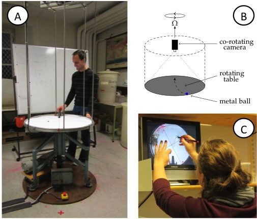
Figure 1A: View of the rotating table. Note the video camera on the scaffolding above the table and the red x (marking the catcher’s position) on the floor in front of the table, diametrically across from where, that very instant, the ball is launched on a ramp. B: Sketch of the rotating table, the mounted (co-rotating) camera, the ramp and the ball on the table. C: Student tracing the curved trajectory of the metal ball on a transparency. On the screen, the experiment is shown as filmed by the co-rotating camera, hence in the rotating frame of reference.

Time needed:

About 45 minutes to one hour per student group. The groups should be sufficiently small so as to ensure active participation of every student. In our small lab space, five has proven to be the upper limit on the number of students per group.

Student task:

In the demonstration, a metal ball is launched from a ramp on a rotating table (Figure 1A,B). Students simultaneously observe the motion from two vantage points: where they are standing in the room, i.e. outside of the rotating system of the table; and, on a screen that displays the table, as captured by a co-rotating camera mounted above it. They are subsequently asked to:

• trace the trajectory seen on the screen on a transparency (Figure 1C),
• measure the radius of this drawn trajectory; and
• compare the trajectory’s radius to the theorized value.

The latter is calculated from the measured rotation rate of the table and the linear velocity of the ball, determined by launching the ball along a straight line on the floor.

Instructional approach

In years prior to 2012, the course had been run along the conventional lines of instruction in an undergraduate physics lab: the students read the instructions, conduct the experiment and write a report.

In 2012, we decided to include an elicit-confront-resolve approach to help students realize and understand the seemingly conflicting observations made from inside versus outside of the rotating system (Figure 2). The three steps we employed are described in detail below.

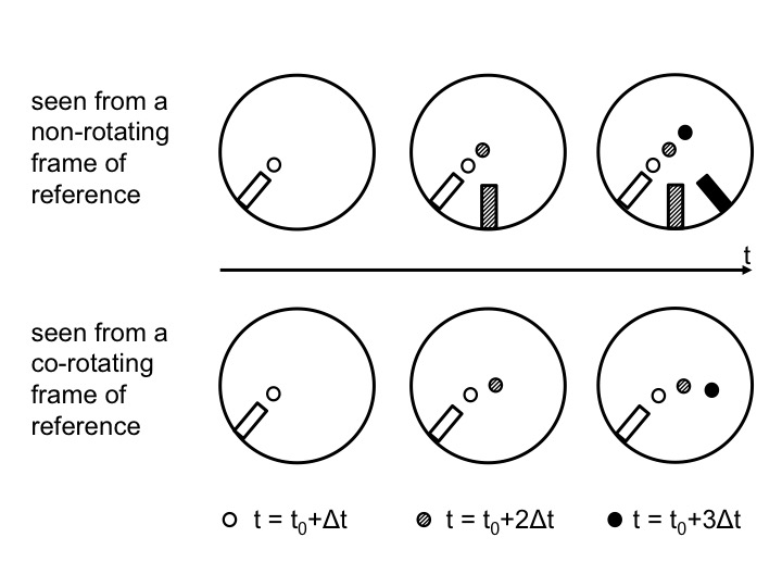
Figure 2: Positions of the ramp and the ball as observed from above in the non-rotating (top) and rotating (bottom) case. Time progresses from left to right. In the top plots, the position in inert space is shown. From left to right, the current position of the ramp and ball are added with gradually darkening colors. In the bottom plots, the ramp stays in the same position, but the ball moves and the current position is always displayed with the darkest color.

1. Elicit the lingering misconception

1.a The general function of the “elicit” step

The goal of this first step is to make students aware of their beliefs of what will happen in a given situation, no matter what those beliefs might be. By discussing what students anticipate to observe under different physical conditions before the actual experiment is conducted, the students’ insights are put to the test. Sketching different scenarios (Fan (2015), Ainsworth et al. (2011)) and trying to answer questions before observing experiments are important steps in the learning process since students are usually unaware of their premises and assumptions. These need to be explicated and verbalized before they can be tested, and either be built on, or, if necessary, overcome.

1.b What the “elicit” step means in the context of our experiment

Students have been taught in introductory lectures that in a counter-clockwise rotating system (i.e. in the Northern Hemisphere) a moving object will be deflected to the right. They are also aware that the extent to which the object is deflected depends on its velocity and the rotational speed of the reference frame.

A typical laboratory session would progress as follows: students are asked to observe the path of a ball being launched from the perimeter of the circular, not-yet rotating table by a student standing at a marked position next to the table, the “launch position”. The ball is observed to be rolling radially towards and over the center point of the table, dropping off the table diametrically opposite from the position from which it was launched. So far nothing surprising. A second student – the catcher – is asked to stand at the position where the ball dropped off the table’s edge so as to catch the ball in the non-rotating case. The position is also marked on the floor with insulation tape.

The students are now asked to predict the behavior of the ball once the table is put into slow rotation. At this point, students typically enquire about the direction of rotation and, when assured that “Northern Hemisphere” counter-clockwise rotation is being applied, their default prediction is that the ball will be deflected to the right. When asked whether the catcher should alter their position, the students commonly answer that the catcher should move some arbitrary angle, but typically less than 90 degrees, clockwise around the table. The question of the influence of an increase in the rotational rate of the table on the catcher’s placement is now posed. “Still further clockwise”, is the usual answer. This then leads to the instructor’s asking whether a rotational speed exists at which the student launching the ball, will also be able to catch it him/herself. Ordinarily the students confirm that such a situation is indeed possible.

2. Confronting the misconception

2.a The general function of the “confront” step

For those cases in which the “elicit” step brought to light assumptions or beliefs that are different from the instructor’s, the “confront” step serves to show the students the discrepancy between what they stated to be true, and what they observe to be true.

2.b What the “confront” step means in the context of our experiment

The students’ predictions are subsequently put to the test by starting with the simple, non-rotating case: the ball is launched and the nominated catcher, positioned diametrically across from the launch position, seizes the ball as it falls off the table’s surface right in front of them. As in the discussion beforehand, the table is then put into rotation at incrementally increasing rates, with the ball being launched from the same position for each of the different rotational speeds. It becomes clear that the catcher need not adjust their position, but can remain standing diametrically opposite to the student launching the ball – the point where the ball drops to the floor. Hence students realize that the movement of the ball relative to the non-rotating laboratory is unaffected by the table’s rotation rate.

This observation appears counterintuitive, since the camera, rotating with the system, shows the curved trajectories the students had expected; circles with radii decreasing as the rotation rate is increased. Furthermore, to add to their confusion, when observed from their positions around the rotating table, the path of the ball on the rotating table appears to show a deflection, too. This is due to the observer’s eye being fooled by focusing on features of the table, e.g. cross hairs drawn on the table’s surface or the bars of the camera scaffold, relative to which the ball does, indeed, follow a curved trajectory. To overcome this latter trickery of the mind, the instructor may ask the students to crouch, diametrically across from the launcher, so that their line of sight is aligned with the table’s surface, i.e. at a zero zenith angle of observation. From this vantage point the ball is observed to indeed be moving in a straight line towards the observer, irrespective of the rate of rotation of the table.

To further cement the concept, the table may again be set into rotation. The launcher and the catcher are now asked to pass the ball to one another by throwing it across the table without it physically making contact with the table’s surface. As expected, the ball moves in a straight line between the launcher and the catcher, who are both observing from an inert frame of reference. However, when viewing the playback of the co-rotating camera, which represents the view from the rotating frame of reference, the trajectory is observed as curved.

3. Resolving the misconception

3.a The general function of the “resolve” step

Misconceptions that were brought to light during the “elicit” step, and whose discrepancy with observations was made clear during the “confront” step, are finally corrected in the “resolve” step. While this sounds very easy, in practice it is anything but. The final step of the elicit-confront-resolve instructional approach thus presents the opportunity for the instructor to aid students in reflecting upon and reassessing previous knowledge, and for learning to take place.

3.b What the “resolve” step means in the context of our experiment

The instructor should by now be able to point out and dispel any remaining implicit assumptions, making it clear that the discrepant trajectories are undoubtedly the product of viewing the motion from different frames of reference. Despite the students’ observations and their participation in the experiment this is not a given, nor does it happen instantaneously. Oftentimes further, detailed discussion is required. Frequently students have to re-run the experiment themselves in different roles (i.e. as launcher as well as catcher) and explicitly state what they are noticing before they trust their observations.

Possible modifications of the activity:

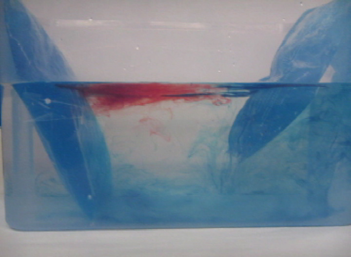
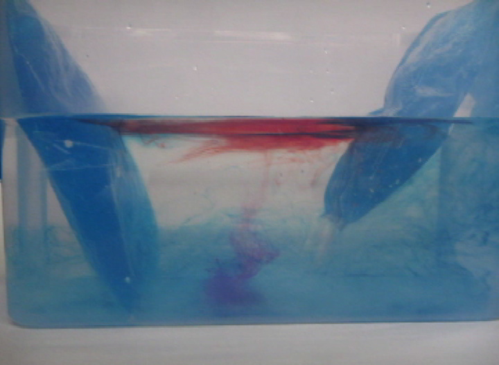
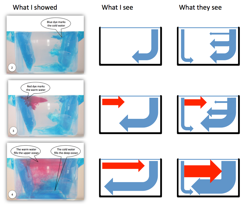
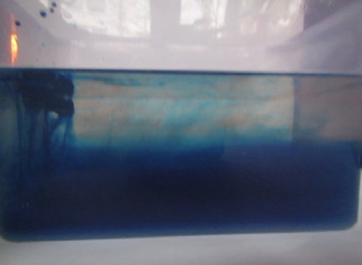
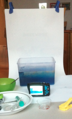
We used the described activity to introduce the laboratory activity, after which the students had to carry out the exercise and write a report about it. Follow-up experiments that are often conducted usually include rotating water tanks to visualize the effect of the Coriolis force on the large-scale circulation of the ocean or atmosphere, for example on vortices, fronts, ocean gyres, Ekman layers, Rossby waves, the General circulation and many other phenomena (see for example Marshall and Plumb (2007)).

Despite their popularity in geophysical fluid dynamics instruction at the authors’ current and previous institutions, rotating tables might not be readily available everywhere. Good instructions for building a rotating table can, for example, be found on the “weather in a tank” website, where there is also the contact information to a supplier given: http://paoc.mit.edu/labguide/apparatus.html. A less expensive setup can be created from old disk players or even Lazy Susans. In many cases, setting the exact rotation rate is not as important as having a qualitative difference between “fast” and “slow” rotation, which is very easy to realize. In cases where a co-rotating camera is not available, by dipping the ball in either dye or chalk dust (or by simply running a pen in a straight line across the rotating surface), the trajectory in the rotating system can be visualized. The method described in this manuscript is easily adapted to such a setup.

Lastly we suggest using an elicit-confront-resolve approach even when the demonstration is not run on an actual rotating table. Even if the demonstration is only virtually conducted, for example using Urbano & Houghton (2006)’s Coriolis force simulation, the approach is beneficial to increasing conceptual understanding.

Discussion

The authors noticed in 2011 that most students participating in that year’s lab course, despite having participated in performing the experiment, still harbored misconceptions. Despite having taken part in performing the demonstration, misunderstanding remained as to what forces were acting on the ball and what the movement of the ball looked like in the different frames of reference. This led to the authors adopting the elicit-confront-resolve approach for instruction, as described above, in 2012.

We initially considered starting the lab session on the Coriolis force by throwing the ball diametrically across the rotating table. Students would then see on-screen the curved trajectory of a ball, which had never made physical contact with the table rotating beneath it. It was thought that initially considering the motion from the co-rotating camera’s view, and seeing it displayed as a curved trajectory when direct observation had shown it to be linear, might hasten the realization that it is the frame of reference that is to blame for the ball’s curved trajectory. However the speed of the ball makes it very difficult to observe its curved path on the screen in real time. Replaying the footage in slow motion helps in this regard. Yet, removing direct observation through recording and playback seemingly hampers acceptance of the occurrence as “real”. It was therefore decided that this method only be used to further illustrate the concept once students were familiar with the general (or standard) experimental setup.

In 2012, 7 groups of 5 students each conducted this experiment under the guidance of both authors together. The authors gained the impression that the new strategy of instruction enhanced the students’ understanding. In order to test this impression and the learning gain resulting from the experiment with the new methodology, in 2013 identical work sheets were administered before and after the experiment. These work sheets were developed by the authors as instructional materials to make sure that every student individually went through the elicit-confront-resolve process even when, with future cohorts, this experiment might be run by other instructors (who might not be as familiar with the elicit-confront-resolve method) and with larger student groups (where individual conversations with every student might be less feasible for the instructor). However, it turned out to be useful for quantifying what we had previously only qualitatively noticed: That a large part of the student population did indeed expect to see a deflection despite observing from an inert frame of reference.

In total, 8 students took the course in 2013, and all agreed to let us talk about their learning process in the context of this article. One of those students did not check the before/after box on the work sheet. We therefore cannot distinguish the work done before and after the experiment, and will disregard this student’s responses in the following discussion. This student however answered correctly on one of the tests and incorrectly on the other.

In the first question, students were instructed to consider both a stationary table and a table rotating at two different rates. They were then asked to, for each of the scenarios, mark with an X the location where they thought the ball would contact the floor after dropping off the table’s surface. In the work sheet done before instruction, all 7 students predicted that the ball would hit the floor in different spots – diametrically across from the launch point for no rotation, and at increasing distances from that first point with increasing rotation rates of the table (Figure 3). This is the same misconception we noticed in earlier years and which we aimed to elicit with this question: students were applying correct knowledge (“In the Northern Hemisphere a moving body will be deflected to the right”) to situations where this knowledge was not applicable (when observing the rotating body and the moving particle upon it from an inert frame of reference).

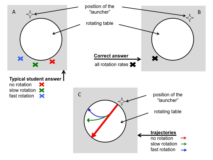
Figure 3A: Depiction of the typical wrong answer to the question where a ball would land on a floor after rolling across a table rotating at different rotation rates. B: Correct answer to question in (A). C: Correct trajectories of balls rolling across a rotating table.

In a second question, students were asked to imagine the ball leaving a dye mark on the table as it rolls across it, and to draw these traces left on the table. In this second question students were thus required to infer that this would be analogous to regarding the motion of the ball as observed from the co-rotating frame of reference. Five students drew them correctly and consistently with the direction of rotation they assumed in the first questions, while the remaining two did not attempt to answer this question.

After the experiment had been run repeatedly and discussed until the students signaled no further need for re-runs or discussion, the students were asked to redo the work sheet. This resulted in 6 students answering both questions correctly. The remaining student answered the second question correctly, but repeated the same incorrect answer to the first question that they gave in their earlier worksheet.

Seeing as the students had extensively discussed and participated in the experiment immediately prior to doing the work sheet for the second time, it is maybe not surprising that the majority answered the questions correctly during the second iteration. In this regard it is important to note that our teaching approach was not planned as a scientific study, but rather developed naturally over the course of instruction. Had we set out to determine the longer-term impact of its efficacy, or its success in abetting conceptual understanding, we should ideally have tested the concept in a new context. As a teaching practice this is advisable.

However, the students’ laboratory reports supply additional support of the claimed usefulness of our new approach. These reports had to be submitted within seven days of originally doing the experiment and accompanying work sheets. One of the questions in their laboratory manual explicitly addresses observing the motion from an inert frame of reference as well as the influence of the table’s rotational period on such motion. This question was answered correctly by all 8 students. This is remarkable for two reasons: firstly, because in the previous year without the elicit-confront-resolve instruction, this question was answered incorrectly by the vast majority of students; and secondly, because for this specific cohort, it is one of the few questions that all students answered correctly in their laboratory reports.

Seven students most certainly make for an insufficient sample size to claim these results have any statistical significance, and this discussion only scratches the surface of what and how students understand frames of reference. However, there is preliminary indication that a) students do indeed harbor the misconception we suspected, and b) that an elicit-confront-resolve approach helped resolve the misunderstanding.

Conclusions

In the suggested instructional strategy, students are required to explicitly state their expectations about what the outcome of an experiment will be, even though their presuppositions are likely to be wrong. The verbalizing of their assumptions aids in making them aware of what they implicitly hold to be true. This is a prerequisite for further discussion and enables confrontation and resolution of potential misconceptions.

This elicit-confront-resolve approach has implications beyond instruction on the Coriolis force or frames of reference. Being able to correctly calculate solutions to textbook problems does not necessarily imply a correct understanding of a concept. Generally speaking, when investigating the roots of student misconceptions, the problem is often located elsewhere than initially suspected. The instructor’s awareness hereof goes a long way towards better understanding and better supporting students’ learning.

We would also like to point out that gaining (the required) insight from a seemingly simple experiment, such as the one discussed in this paper, might not be nearly as straightforward or obvious for the students as anticipated by the instructor. Again, probing for conceptual understanding rather than the ability to calculate a correct answer proved critical in understanding where the difficulties stemmed from, and only a detailed discussion with several students could reveal the scope of difficulties. We would encourage every instructor not to take at face value the level of difficulty your predecessors claim an experiment to have!

Acknowledgements

The authors are grateful for the students’ consent to present their worksheet responses in this article.

Supplementary materials

Movies of the experiment can be seen here:

Rotating case: https://vimeo.com/59891323

Non-rotating case: https://vimeo.com/59891020

References

Ainsworth, S., Prain, V., & Tytler, R. (2011). Drawing to Learn in Science Science, 333 (6046), 1096-1097 DOI: 10.1126/science.1204153

Baillie, C., MacNish, C., Tavner, A., Trevelyan, J., Royle, G., Hesterman, D., Leggoe, J., Guzzomi, A., Oldham, C., Hardin, M., Henry, J., Scott, N., and Doherty, J. 2012. Engineering Thresholds: an approach to curriculum renewal. Integrated Engineering Foundation Threshold Concept Inventory 2012. The University of Western Australia, < http://www.ecm.uwa.edu.au/__data/assets/pdf_file/0018/2161107/Foundation-Engineering-Threshold-Concept-Inventory-120807.pdf>

Coriolis, G. G. 1835. Sur les équations du mouvement relatif des systèmes de corps. J. de l’Ecole royale polytechnique 15: 144–154.

Cushman-Roisin, B. 1994. Introduction to Geophysical Fluid DynamicsPrentice-Hall. Englewood Cliffs, NJ, 7632.

Durran, D. R. and Domonkos, S. K. 1996. An apparatus for demonstrating the inertial oscillation, BAMS, Vol 77, No 3

Fan, J. (2015). Drawing to learn: How producing graphical representations enhances scientific thinking. Translational Issues in Psychological Science, 1 (2), 170-181 DOI: 10.1037/tps0000037

Gill, A. E. 1982. Atmosphere-ocean dynamics (Vol. 30). Academic Pr.

Kornell, N., Jensen Hays, M., and Bjork, R.A. (2009), Unsuccessful Retrieval Attempts Enhance Subsequent Learning, Journal of Experimental Psychology: Learning, Memory, and Cognition 2009, Vol. 35, No. 4, 989–998

Hart, C., Mulhall, P., Berry, A., Loughran, J., and Gunstone, R. 2000. What is the purpose of this experiment? Or can students learn something from doing experiments?, Journal of Research in Science Teaching, 37 (7), p 655–675

Mackin, K.J., Cook-Smith, N., Illari, L., Marshall, J., and Sadler, P. 2012. The Effectiveness of Rotating Tank Experiments in Teaching Undergraduate Courses in Atmospheres, Oceans, and Climate Sciences, Journal of Geoscience Education, 67–82

Marshall, J. and Plumb, R.A. 2007. Atmosphere, Ocean and Climate Dynamics, 1^st Edition, Academic Press

McDermott, L. C. 1991. Millikan Lecture 1990: What we teach and what is learned – closing the gap, Am. J. Phys. 59 (4)

Milner-Bolotin, M., Kotlicki A., Rieger G. 2007. Can students learn from lecture demonstrations? The role and place of Interactive Lecture Experiments in large introductory science courses. The Journal of College Science Teaching, Jan-Feb, p.45-49.

Muller, D.A., Bewes, J., Sharma, M.D. and Reimann P. 2007. Saying the wrong thing: improving learning with multimedia by including misconceptions, Journal of Computer Assisted Learning (2008), 24, 144–155

Newcomer, J.L. 2010. Inconsistencies in Students’ Approaches to Solving Problems in Engineering Statics, 40th ASEE/IEEE Frontiers in Education Conference, October 27-30, 2010, Washington, DC

Persson, A. 1998. How do we understand the Coriolis force?, BAMS, Vol 79, No 7

Persson, A. 2010. Mathematics versus common sense: the problem of how to communicate dynamic meteorology, Meteorol. Appl. 17: 236–242

Pinet, P. R. 2009. Invitation to oceanography. Jones & Bartlett Learning.

Posner, G.J., Strike, K.A., Hewson, P.W. and Gertzog, W.A. 1982. Accommodation of a Scientific Conception: Toward a Theory of Conceptual Change. Science Education 66(2); 211-227

Pond, S. and G. L. Pickard 1983. Introductory dynamical oceanography. Gulf Professional Publishing.

Roth, W.-M., McRobbie, C.J., Lucas^, K.B., and Boutonné, S. 1997. Why May Students Fail to Learn from Demonstrations? A Social Practice Perspective on Learning in Physics. Journal of Research in Science Teaching, 34(5), page 509–533

Talley, L. D., G. L. Pickard, W. J. Emery and J. H. Swift 2011. Descriptive physical oceanography: An introduction. Academic Press.

Tomczak, M., and Godfrey, J. S. 2003. Regional oceanography: an introduction. Daya Books.

Trujillo, A. P., and Thurman, H. V. 2013. Essentials of Oceanography, Prentice Hall; 11 edition (January 14, 2013)

Urbano, L.D., Houghton J.L., 2006. An interactive computer model for Coriolis demonstrations. Journal of Geoscience Education 54(1): 54-60

—

P.S.: This text originally appeared on my website as a page. Due to upcoming restructuring of this website, I am reposting it as a blog post. This is the original version last modified on January 24th, 2017.