Tag: overturning

Thermal forcing vs rotation tank experiments in more detail than you ever wanted to know
This is the long version of the two full “low latitude, laminar, tropical Hadley circulation” and “baroclinic instability, eddying, extra-tropical circulation” experiments. A much shorter version (that also includes the…
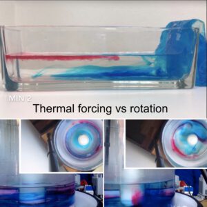
Thermal forcing vs rotation
The first experiment we ever ran with our DIYnamics rotating tank was using a cold beer bottle in the center of a rotating tank full or lukewarm water. This experiment is…
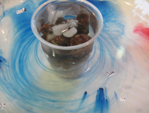
Brine rejection and overturning, but not the way you think! Guest post by Robert Dellinger
It’s #KitchenOceanography season! For example in Prof. Tessa M Hill‘s class at UC Davis. Last week, her student Robert Dellinger posted a video of an overturning circulation on Twitter that got me…
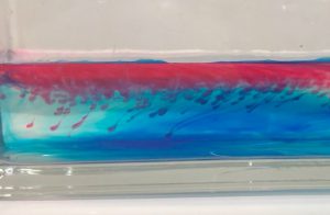
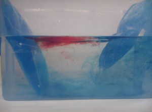
Salt fingers in my overturning experiment
You might have noticed them in yesterday’s thermally driven overturning video: salt fingers! In the image below you see them developing in the far left: Little red dye plumes moving…
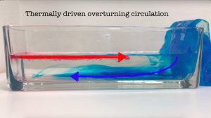
Thermally driven overturning circulation
Today was the second day of tank experiments in Torge’s and my “dry theory 2 juicy reality” teaching innovation project. While that project is mainly about bringing rotating tanks into…
Combining a slowly rotating water tank with a temperature gradient: A thermal wind demonstration!
Setting up an overturning circulation in a tank is easy, and also interpreting the observations is fairly straightforward. Just by introducing cooling on one side of a rectangular tank a…
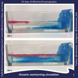
Experiment: Oceanic overturning circulation (the slightly more complicated version)
The experiment presented on this page is called the “slightly more complicated version” because it builds on the experiment “oceanic overturning circulation (the easiest version)” here. Background One of the…
Experiment: Oceanic overturning circulation (the easiest version)
“The easiest” in the title of this page is to show the contrast to a “slightly more complicated” version here. Background One of the first concepts people hear about in the context…
Temperature-driven overturning experiment – the easy way
In my last post, I showed you the legendary overturning experiment. And guess what occurred to me? That there is an even easier way to show the same thing. No gel…
A very simple overturning experiment for outreach and teaching
For one of my side-projects I needed higher-resolution photos of the overturning experiment, so I had to redo it. Figured I’d share them with you, too. You know the experiment: gel…
Thermally-driven overturning circulation
Cooling on one end of the tank, heating on the other: A temperature-driven overturning. [deutscher Text unten] Always one of my favorite experiments – the overturning experiment (and more, and more).…
An overturning experiment (part 3)
By popular demand: A step-by-step description of the overturning experiment discussed here and here. I wrote this description a while ago and can’t be bothered to transfer it into the…
An overturning experiment (part 2)
How to adapt the same experiment to different levels of prior knowledge. In this post, I presented an experiment that I have run in a primary school, with high-school pupils,…
An overturning experiment
A simple experiment that shows how the large-scale thermally-driven ocean circulation works. Someone recently asked me whether I had ideas for experiments for her course in ocean sciences for non-majors.…