Tag Archives: salinity

Salt fingering

How to show my favorite oceanographic process in class, and why.

As I mentioned in this post, I have used double-diffusive mixing extensively in my teaching. For several reasons: Firstly, I think that the process is just really cool (watch the movie in this post and tell me that it isn’t!!!) and that the experiments are neat and that everybody will surely be as excited about them as I am. Secondly, because it shows that understanding of small processes can be really important in order to understand the whole eco- and even climate system. And thirdly, because it helps to demonstrate a way of thinking about oceanography.

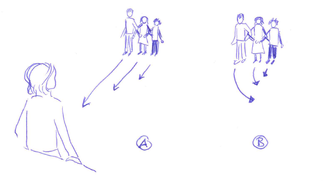
When I introduce salt fingering, I talk students through the process in very small steps. It goes something like this (Numbering is referring to the sketch below):

1) Initially, you have a stratification where warm and salty overlies cold and fresh water. This stratification is stable in density (meaning the influence of the temperature stratification on density outweighs that of the salinity stratification).

2) Since molecular diffusion of temperature is about a factor 100 faster than that of salinity (we will talk about why that is in a later blog post), the interface in salinity is initially basically unchanged, whereas a temperature exchange is happening across that interface, and a layer of medium temperature is forming.

3) At the salinity interface, we now have a stratification that is no longer stable in density: while the water now has the same temperature in a thin layer above and below the interface, it is still more salty on top and less salty below the interface. This means that the saltier water in this thin layer is denser than the less salty water below. This leads to finger-shaped instabilities at the interface: The salty water will sink and the fresh water will rise.

The individual salt fingers now have a much larger surface than the original interface, hence molecular diffusion of salt will happen much more efficiently and eventually the salinity inside and outside of the salt fingers will be the same, hence the growth of the fingers will stop.

At the depth where the salt fingers stopped, a new interface has formed. This new interface can also develop salt fingering, leading to a staircase-like structure in temperature and salinity.

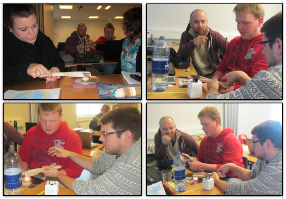
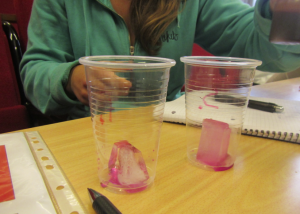
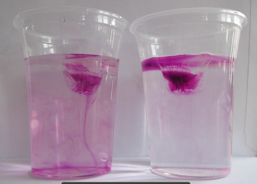
After salt fingering has been introduced, there are usually several other occasions where it, or its effects, can be pointed out, like for example when showing this experiment (see picture below), when talking about the hydrographic properties in the area of the Mediterranean outflow or the Arctic, or when talking about nutrients in subtropical gyres.

IMG_4233_sehr_klein

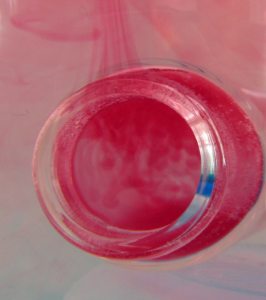
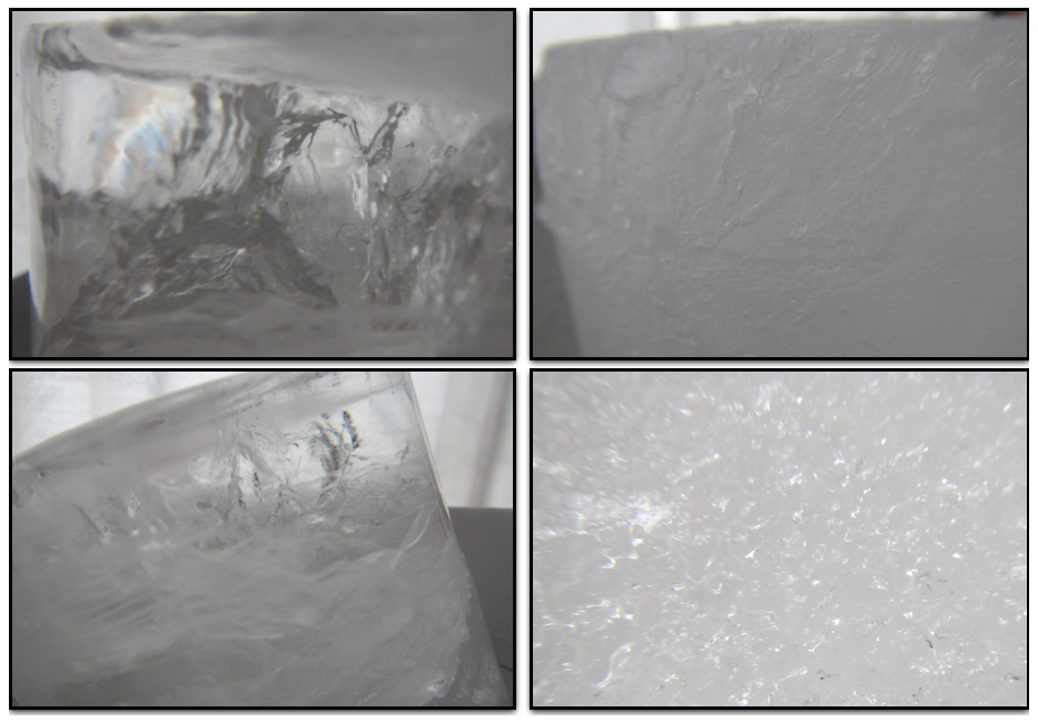
This is a zoom in on one of the bottles shown in this experiment: In the warm bottle, the red food dye acts as salt to form salt fingers!

While talking about salt fingering, since I focus so much on the process, I have always been under the illusion that students actually understand the reasoning behind it and that they can reproduce and transfer it. Reproduce they can – transfer not so much. Stay tuned for the next post discussing reasons and possible ways around it.

Double-diffusive mixing

On the coolest process in oceanography.

My favorite oceanographic process, as all of my students and many of my acquaintances know, is double-diffusive mixing. Look at how awesome it is:

Double-diffusive mixing happens because heat and salt’s molecular diffusion are very different: Heat diffuses about a factor 100 faster than salt. This can lead to curious phenomena: Bodies of water with a stable stratification in density will start to mix much more efficiently than one would have thought.

In the specific case of a stable density stratification with warm, salty water over cold, fresh water, finger-like structures form. Those structures are called “salt fingers”, the process is “salt fingering”.

IMG_4233_sehr_klein

Salt fingering happening with the red food dye acting as “salt”.

Even though salt fingers are tiny compared to the dimensions of the ocean, they still have a measurable effect on the oceanic stratification in the form of large-scale layers and stair cases, and not only the stratification in temperature and salinity, but also on nutrient availability in the subtropical gyres, for example, or on CO2 drawdown.

Over the next couple of posts, I will focus on double diffusive mixing, but less on the science and more on how it can be used in teaching. (If you want to know more about the science, there are tons of interesting papers around, for example my very first paper)

How sound is refracted towards the regions of minimum speed.

Students acting out the process of sound being refracted towards the region of minimum speed.

We’ve been talking about refraction lately. Waves get bent in the direction of lower velocity. This holds for light and sound and even ocean waves. However, students find it conceptually difficult to understand why waves are being bent towards lower rather than higher speeds, so I came up with this very simple demonstration.

Students, arms joint, are acting as a wave crest. Students on the one side of the student chain are told to move very slowly, students on the other side are asked to move quickly towards the instructor. Everybody takes care to not hurt anybody, so if tension builds up in the chain, everybody has to react to reduce the tension. What happens is that the “wave crest” of students changes direction towards the side of the slowest motion.

Easy visualization and – since it involved students getting up, joining arms and doing something – also very memorable. Win – win!

Another easy example: When you are sliding on an icy road and your foot gets caught in grass or gravel or something on one side (== region of lower velocity), you start skidding towards the side with the obstacle, not towards the middle of the icy road.

Measuring salinity

Students evaporate water to measure the salinity of a water sample.

As described in this post, I like to have students build “instruments” to measure the most oceanographic properties (temperature, salinity and density). I find that they appreciate oceanographic data much more once they have first-hand experience with how difficult it is to design instruments and make sense of the readings. Today I’m presenting two groups that focused on salinity, while yesterday’s group was measuring density.

Students evaporate water to measure the salinity of a water sample.

The students in the course I currently teach were determined to not only evaporate some water to qualitatively look at how much salt was dissolved in the sample, they wanted to do it right. So they set out to measure the vessel, the sample and the remaining salt. But since measuring salinity is really pretty difficult, they ran into a couple of problems. First – my scales were nowhere near good enough to measure the amount of water they could fit into the evaporation cup with any kind of precision. Second, even the amount of water that they could fit took a lot longer to evaporate (or even boil) than anticipated. Third, they realized that even though they could see salt residue in the end, this might not be all the salt that had been there in the beginning, plus there was grime accumulating at the base of the cup, so weighing the cup in the end might not be the best option. But they still learned a lot from that experiment: For example that once the (small quantity of) water was boiling, it became milky very quickly and then turned to crystallized salt almost instantly. Or that in order to use this method, a tea candle is not as suitable as a heat source as a lighter (and there might probably even be even better ones out there).

P.S.: In this course, none of the groups set the wooden tongs on fire! :-)

Tasting sea water reloaded

Doing the “tasting sea water” activity again with a different group of students.

A very good introduction to the concept of salinity is the “tasting sea water” activity. Last time I ran that activity, students were very quick to correctly connect the samples with the correct sampling locations without much discussion going on. This time round, though, there was a lot of discussion. Students quickly sorted samples in order of increasing salinity, but there was no agreement to be found on whether the Baltic or the Arctic should be fresher. Since I only pointed to a location and didn’t specify the depth at which the sample had been taken, some students argued that the Arctic was very fresh at the very top, whereas the Baltic was brackish. Others said that the Baltic was a lot fresher than any oceanic location.

salt-tasting

Students tasting four different samples of “sea water” with salinities corresponding to Arctic sea ice, the Baltic sea, the open ocean and the Mediterranean. Samples have to be associated with locations on a map.

In another group, there was a big discussion going on about how in marginal seas, evaporation or precipitation can dominate.

It is always great to see how much you can discuss and learn from an activity as simple as this one!

How a CTD works

Movie on how the most important instrument in oceanography works.

On our cruise on the WHOI research vessel Knorr in 2011, Sindre Skrede (find him on twitter or vimeo for many more exciting pictures and movies!) and I made a movie for his blog, describing the most important oceanographic instrument. We recently translated the movie from Norwegian to English and here it is. Enjoy!

On the structure of fresh water and salt water ice

More details on the structure of fresh water and salt water ice.

Fresh water and salt water ice have very different structures as I already discussed in this post.

Fresh water ice (on the left) and salt water ice (on the right).

In the image above you see that the structures are very different. Whereas fresh water ice is clear and transparent, salt water ice has a porous structure and is milky.

Investigating fresh water and salt water ice cubes in class. Already in this photo the difference is clearly visible, and it is even more obvious when you pick up the cups and look at the ice cubes from the side.

The pores can be made visible by dropping dye on the ice cubes, as we did in class on Tuesday. For salt water ice, dye penetrates into the ice cube along the brine channels; the ice cube seems to be soaking up the dye like a sponge and becomes colored through and through. In case of the fresh water ice, dye cannot penetrate because the crystal structure is so regular and tight, and the dye just comes off the ice.

Melting ice cubes – one experiment, many ways (post 3/4)

Different didactical settings in which the “ice cubes melting in fresh and salt water” experiment can be used.

In part 1 and 2 of this series, I showed two different ways of using the “ice cubes melting in fresh water and salt water” experiment in lectures. Today I want to back up a little bit and discuss reasons for choosing one over the other version in different contexts.

Depending on the purpose, there are several ways of framing this experiment. This is very nicely discussed in materials from the Lawrence Hall of Science (link here), too, even though my discussion is a little different from theirs.

1) A demonstration.

If you want to show this experiment rather than having students conduct it themselves, using colored ice cubes is the way to go (see experiment here). The dye focuses the observer’s attention on the melt water and makes it much easier to observe the experiment from a distance, on a screen or via a projector. Dying the ice cubes makes understanding much easier, but it also diminishes the feeling of exploration a lot – there is no mystery involved any more.

Demonstration of melting ice cubes. The melt water is clearly marked by the dye. This makes it a good demonstration, but diminishes the satisfying feeling of discovery by the observer, because the processes are clearly visible right away rather than having to be explored.

2) A structured activity.

Students are handed (non-colored) ice cubes, cups with salt water and fresh water and are asked to make a prediction about which of the ice cubes is going to melt faster. Students test their hypothesis, find the results of the experiment in support with it or not, and we discuss. This is how I usually use this experiment in class (see discussion here).

The advantage of using this approach is that students have clear instructions that they can easily follow. Depending on how observant the group is, instructions can be very detailed (“Start the stop watch when you put the ice cubes in the water. Write down the time when the first ice cube has melted completely, and which of the ice cubes it was. Write down the time when the second ice cube has melted completely. …”) or more open (“observe the ice cubes melting”).

3) A problem-solving exercise.

In this case, students are given the materials, but they are not told which of the cups contains fresh or salt water (and they are instructed not to taste). Now students are asked to design an experiment to figure out which cup contains what.

This is a very nice exercise and students learn a lot from designing the experiment themselves. However, this also takes a very long time, more than I can usually afford to spend on experiments in class. After all, I am doing at least one hands-on activity in each of the lectures, but am still covering the same content from the text book as previous lecturers who used their 180 minutes per week just lecturing. And I am considering completely flipping my class room, but I am not there yet.

4) An open-ended investigation.

In this case, students are handed the materials, knowing which cup contains fresh and salt water. But instead of being asked a specific question, they are told to use the materials to learn as much as they can about salt water, fresh water, temperature and density.

As with the problem-solving exercise, this is a very time-intensive undertaking that does not seem feasible in the framework we are operating in. Also it is hard to predict what kind of experiments the students will come up with, and if they will learn what you want them to learn. On the other hand, students typically learn much more because they are free to explore and not bound by a specific instruction from you.

How much salt is there in sea water?

Visualization of how much salt is actually contained in sea water.

When preparing “sea water samples” for class, it is always astonishing to me how much salt I have to add for normal open-ocean salinities. Time and time again it looks like it should be way too much, but then when tasting it, it tastes salty, but like the ocean and not like brine.

A teaspoon full of salt corresponds to approximately 5 grams. That means that for typical open-ocean salinities, you have to add 7 teaspoons full of salt to a liter of water.

Since it is still astonishing to us, Pierre and I thought, it would probably be a good thing to show to our students. 0.18 teaspoon full of salt corresponds to only 1 gram of salt (averaged over several non-scientific internet sources, but well within the measurement error of my kitchen scales [and yes, I know the trick of measuring the weight of several spoons and then dividing by the number, but thanks!]).

What I want to do in the lecture is have the students estimate how much salt they need for a 35 psu liter of water. And not estimate by weighing (because I want each of the students to be able to touch the salt, but at the same time don’t want salt all over the lecture theatre), but visually estimate.

10 grams of salt in a little plastic jar.

The little jar in the picture above contains 10 grams of salt. So in order to have students estimate how much salt they would need for a liter of 35psu water, we filled 12 of those little jars with 10 grams each and handed them to the students. Obviously we didn’t tell the students how much salt was contained in a jar!

12 x 10 grams of salt. It does look like a lot more, doesn’t it?

Knowing that there are 10 grams of salt in each of the jars, it is pretty obvious that we need three and a half of those little jars for 35 grams of salt. When we did this in the lecture on Tuesday – and again, the students were not told how much salt was in one jar! -, the first person who answered guessed “four”. And then someone actually said “three and a half”. Oh well, lucky guess or great skill? I was hoping for answers like “maybe one of those jars”, because that would be closer to my own intuition. I guess next time I’ll be framing it differently. Maybe use something with one liter volume and put 35 grams in it? Or ask them to tell me in teaspoons? Does anyone have a good idea that they would like to share with me?

Properties of sea ice and fresh water ice

Sea ice and fresh water ice have distinctly different properties that can easily be investigated even in big class rooms.

In “on how ice freezes from salt water” I talked a bit about how dye was rejected when I tried to produce colored ice cubes for another experiment. But even non-colored ice that were made out of fresh water or salt water shows distinctly different structures.

Ice formed from fresh water (on the left) and salt water (on the right). Note the small pores in the salt water ice cube – those are the channels that form when brine is rejected.

On the left, you see that the surface is very smooth apart from a couple of cracks. The red food dye that was dripped on the ice cube comes right off, like water off a duck’s back. On the right, the food coloring is not rolling off, instead it is creeping into all the little brine channels, hence nicely showing a web of pores all throughout the ice cube.

I first saw this experiment when Angelika Renner from the Norwegian Polar Institute in Tromsø visited my GEOF130 class last year. She says that she got the idea from the APECS book [link*], that, btw, provides many great ideas for outreach projects.

* I’m not affiliated, nor do I get money for recommending this book. It’s just a great resource that I think everybody should be aware of!

[edit 11.9.2013: new post on the same topic here: http://mirjamglessmer.com/2013/09/11/on-the-structure-of-fresh-water-and-salt-water-ice/]