I could watch flow fields for the rest of my life and not get bored :-)
Eddy formation from shear instabilities
Eddy formation from shear instabilities
I could watch flow fields for the rest of my life and not get bored :-)
Eddy formation from shear instabilities
Eddy formation from shear instabilities
I just realized we never showed you that you can see the Coriolis deflection on the inflowing water when we started filling the tank! So here you go. Isn’t that cool? (Remember, we are in the Southern Hemisphere…)
Coriolis deflection of water flowing into the tank during filling
Kelvin-Helmholtz instabilities
Don’t you just love watching this kind of stuff? :-)
Kelvin-Helmholtz instabilities
What happens when the almost neutrally buoyant particles that we use to visualize the flow field have sunken out of the surface layer?
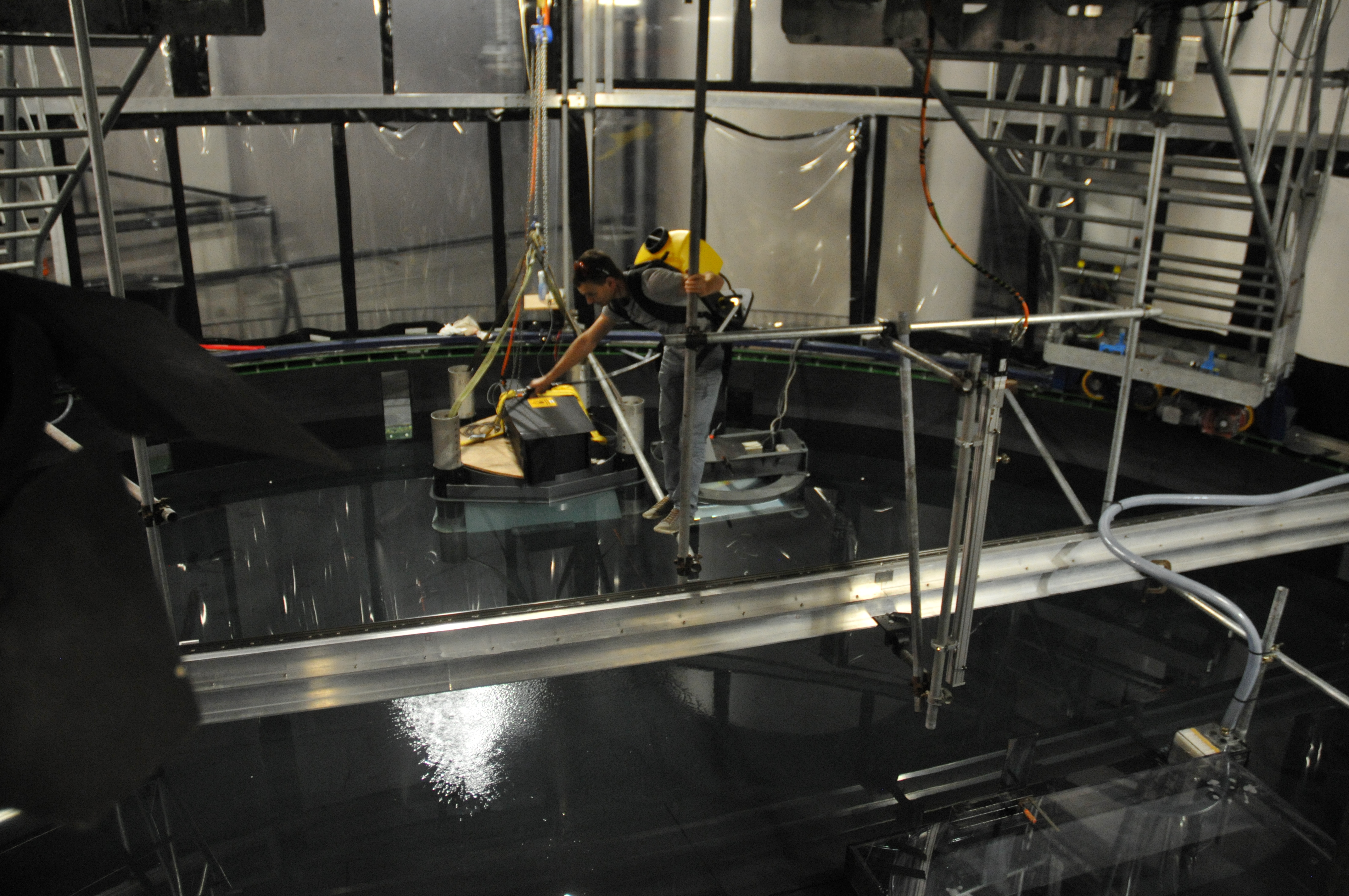
And this is how the particles are added into the tank!
The fairy-dust sprinkler comes and sprinkles more fairy dust! :-)
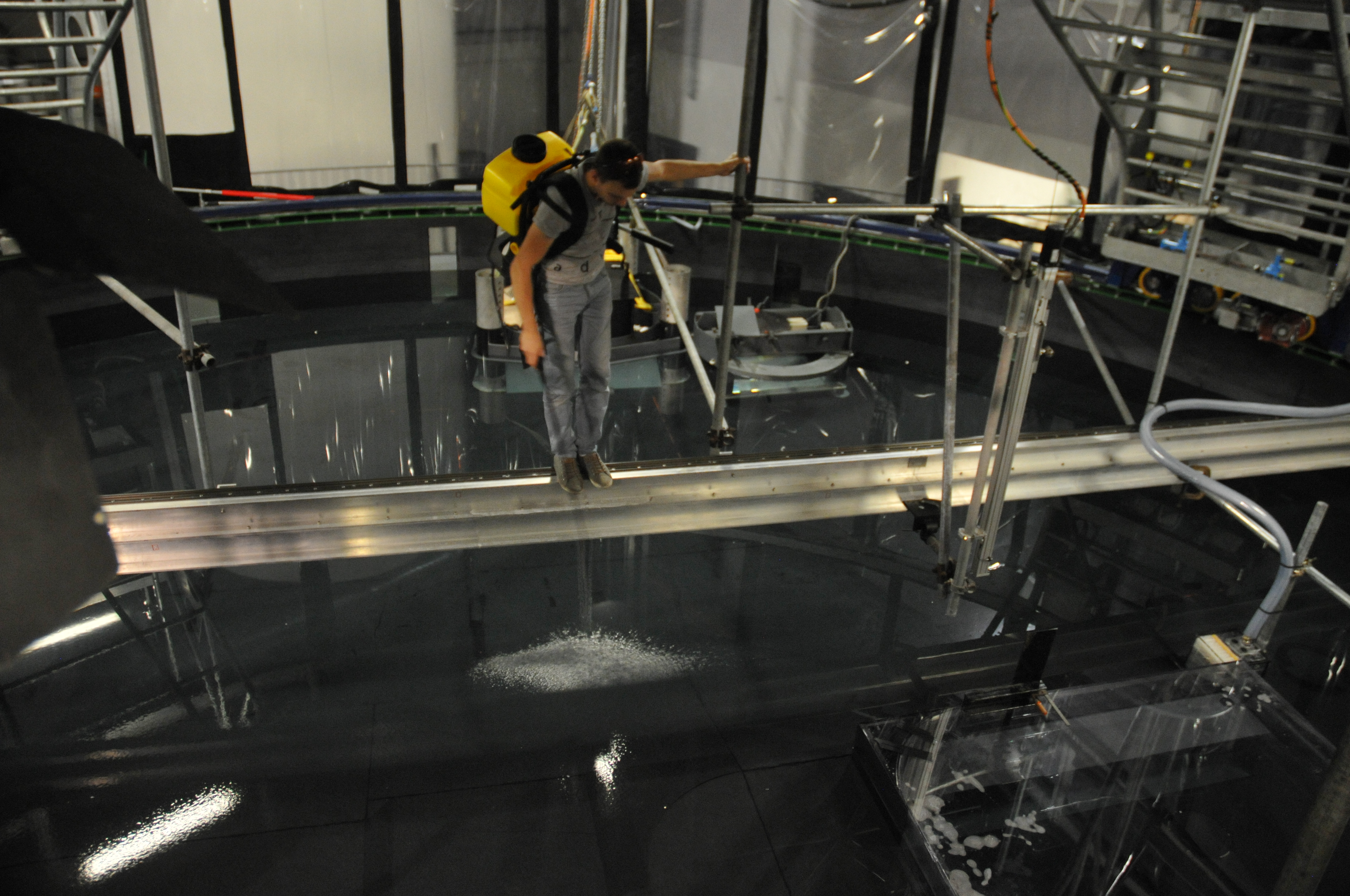
Thomas adding more particles
And that produces all these cute little swirls that glow bright green. So pretty! :-)
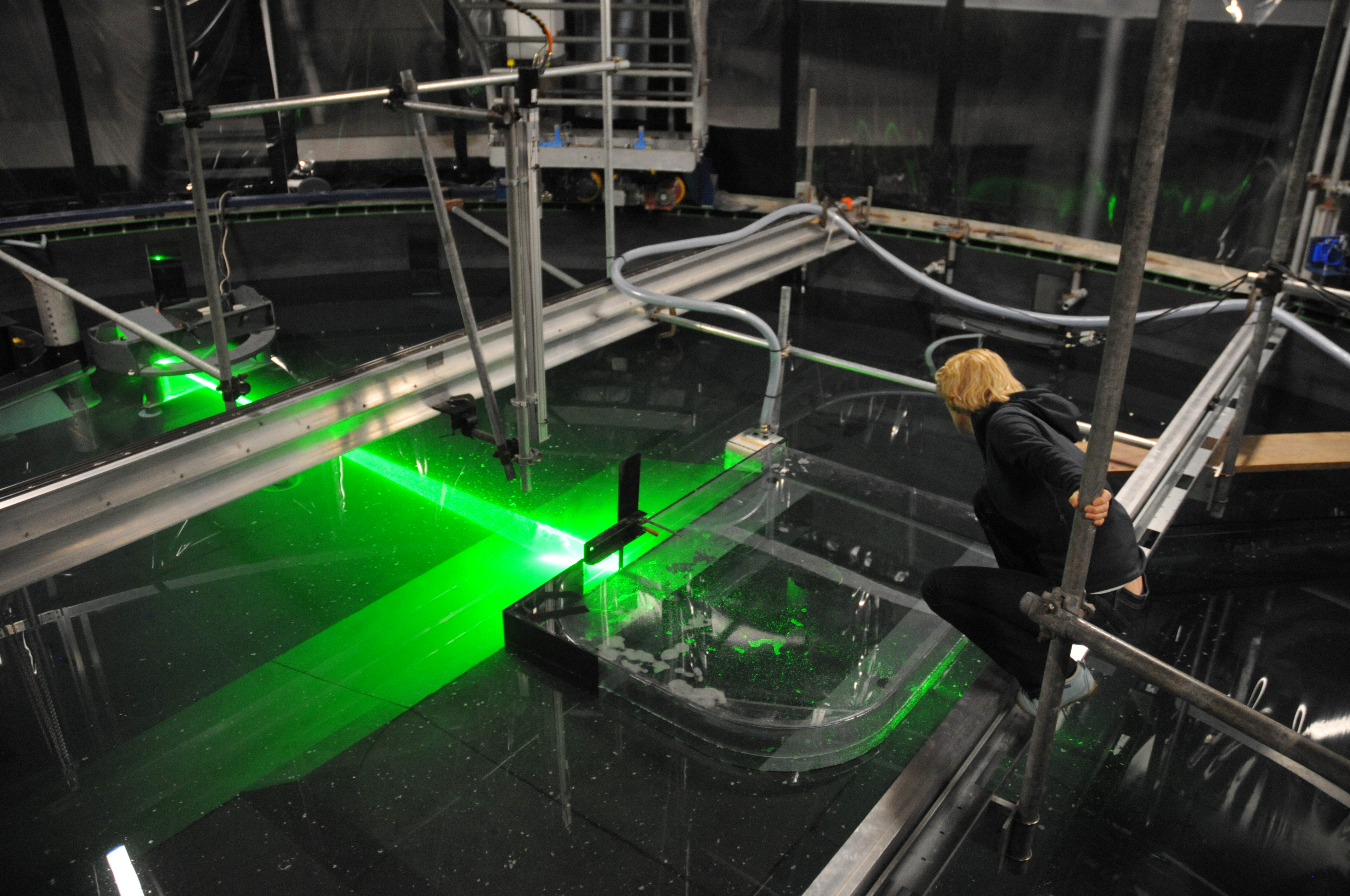
Elin observing Antarctic currents close up and personal
We’ve talked before how we use the laser to light up neutrally-buoyant particles on horizontal slices of our tank, but we can actually also do this in the vertical.
Elin and Thomas observing Samuel working on the laser
This is sometimes very helpful to check whether the particle distribution is still good enough or whether someone needs to go in and stir up some particles before the next experiment.
Can you see the particles in the current?
You’ve probably been wondering about this, too: We have a constant inflow from our “source” into the tank. How do we keep the water level stable?
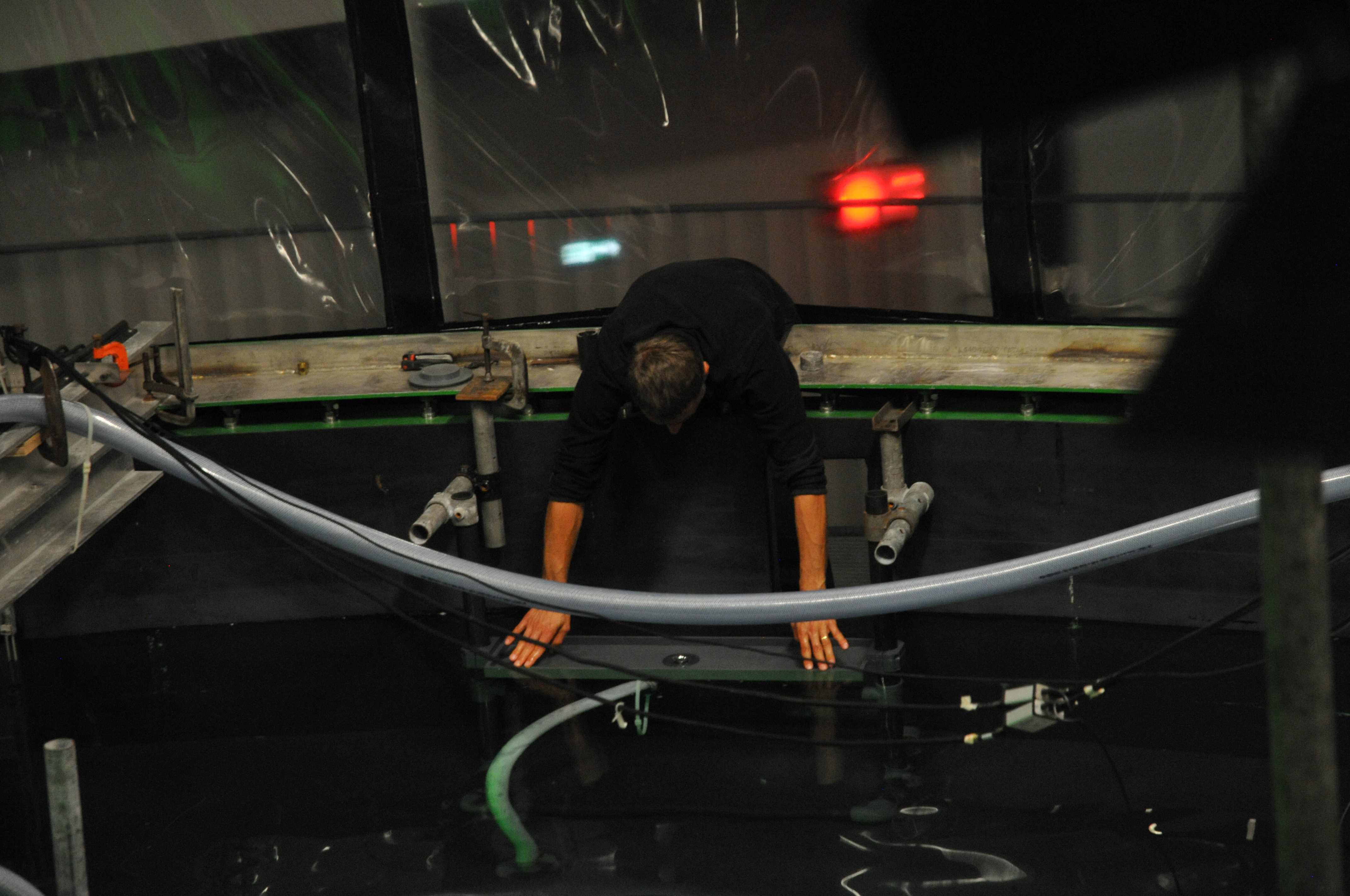
Samuel adjusting the “skimmer” to regulate the outflow of the tank
Worry no more — here is the answer. In the picture above you see Samuel adjusting the skimmer — a sink inside the tank that height is adjusted such that its upper edge is exactly at where the water level should be. So any excess water is skimmed off and drained.
Sounds easy, but it’s actually not — we have a free surface in the tank and we are rotating quite fast, so there is a height difference of almost 10 cm between the center and the outer edge. So a little bit of fiddling around involved…
Just so you don’t get bored over the weekend (and because they are so so beautiful to look at!) here are a couple more sneak peek gifs of our experiments.
Remember, though, that what we see are only particle distributions in one layer close to the surface, and also the very beginning of the experiments before the flow has reached a balance. So please don’t over-interpret :-)
This blog post was written for Elin Darelius & team’s blog (link). Check it out if you aren’t already following it!
—
I read a blog post by Clemens Spensberger over at a scisnack.com couple of years ago, where he talks about how ice can flow like ketchup. The argument that he makes is that ketchup on your hotdog behaves in many ways similarly to glaciers on for example Greenland: If there is a layer of a certain thickness, it will start sliding off — both the ketchup off your hotdog and the glaciers off Greenland. After most of it has dripped to your shirt or in the ocean, a little bit still remains on the hotdog or the mountain. And so on.
What he is talking about, basically, are effects of viscosity. Water, for example, would behave very differently than ketchup or ice, if you imagine it poured on your hotdog or raining down on Greenland. But also ketchup would behave very differently from ice, if it was put on Greenland in the same quantities as the existing glaciers on Greenland, instead of on a hotdog as a model version of Greenland in a relatively small quantity. And if you used real ice to model the behaviour of Greenland glaciers on a desk, then you would quickly find out that the ice just slides off on a layer of melt water and behaves nothing like you imagined (ask me how I know…).
This shows that it is important to think about what role viscosity plays when you set up a model. And not only when you are thinking about ice — also effects of surface tension in water become very important if your model is small enough, whereas they are negligible for large scale flows in the ocean.
The effects of viscosity can be estimated using the Reynolds number Re. Re compares the effects of the velocity u of the flow, a length scale of an obstacle L, and the viscosity v: Re = uL/v.
Reynolds numbers can be used to separate different flow regimes: laminar flows for very low Reynolds numbers, nice vortex streets for Re > 90, and then flows with a stagnant backwater for high Reynold numbers.
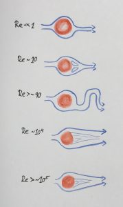
Dependency of a flow field on the Reynolds number. Shown is the top view of a flow field. You see red obstacles and blue stream lines (so any particle released at any point of a blue line would follow that line exactly, and in the direction shown by the arrow heads)
I have thought long and hard about what I could give as a good example for what I am talking about. And then I remembered that I did an experiment on vortex streets on a plate a while back.
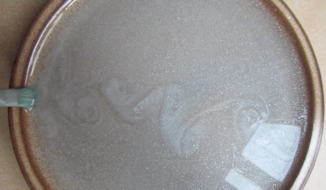
Vortices created on a plate
If you start watching the movie below at min 1:28 (although watching before won’t hurt, either) you see me pulling a paint brush across the plate at different speeds. The slow ones don’t create vortex streets, instead they show a more laminar behaviour (as they should, according to theory).
Vortex streets, like the one shown in the picture above, also exist in nature. However, scales are a lot larger there: See for example the picture below (Credit: Bob Cahalan, NASA GSFC, via Wikipedia)

Vortex street. Credit: Bob Cahalan, NASA GSFC, via Wikipedia
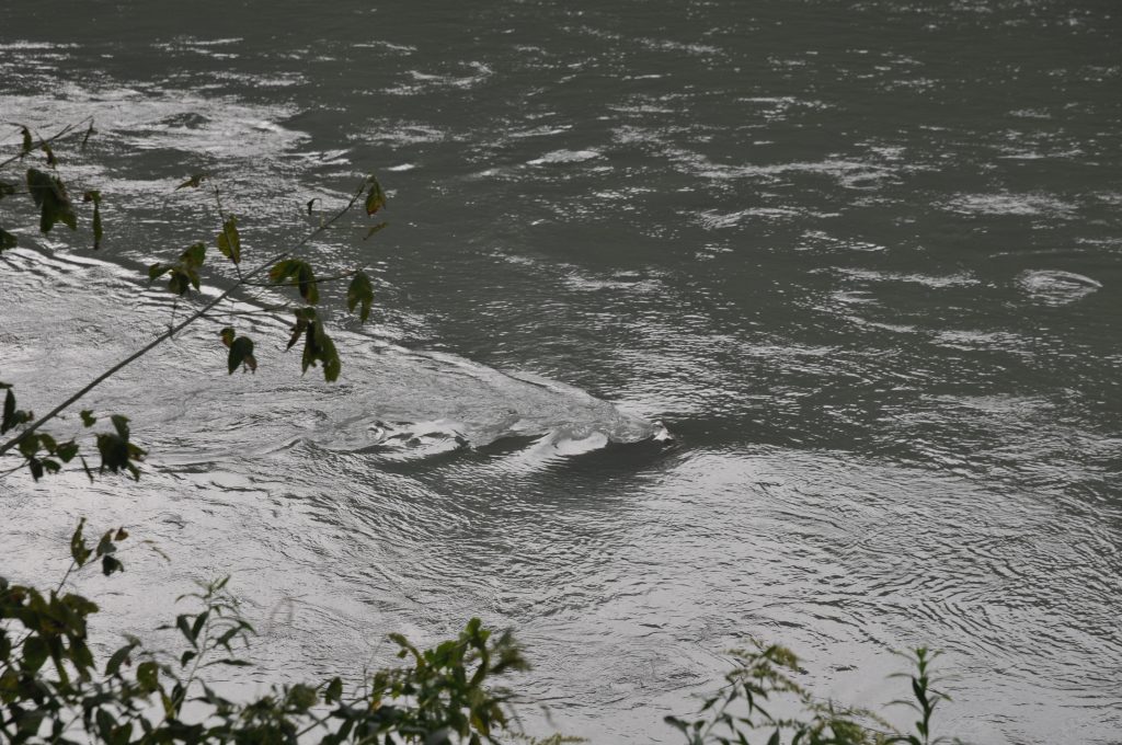
While this is a very distinctive flow that exists at a specific range of Reynolds numbers, you see flows of all different kinds of Reynold numbers in the real world, too, and not only on my plate. Below, for example, the Reynolds number is higher and the flow downstream of the obstacle distinctly more turbulent than in a vortex street. It’s a little difficult to compare it to the drawing of streamlines above, though, because the standing waves disguise the flow.
One way to manipulate the Reynolds number to achieve similarity between the real world and a model is to manipulate the viscosity. However that is not an easy task: if you wanted to scale down an ocean basin into a normal-sized tank, you would need fluids to replace the water that don’t even exist in nature in liquid form at reasonable temperatures.
All the more reason to use a large tank! :-)
A very convenient way to describe a flow system is by looking at its Froude number. The Froude number gives the ratio between the speed a fluid is moving at, and the phase velocity of waves travelling on that fluid. And if we want to represent some real world situation at a smaller scale in a tank, we need to have the same Froude numbers in the same regions of the flow.
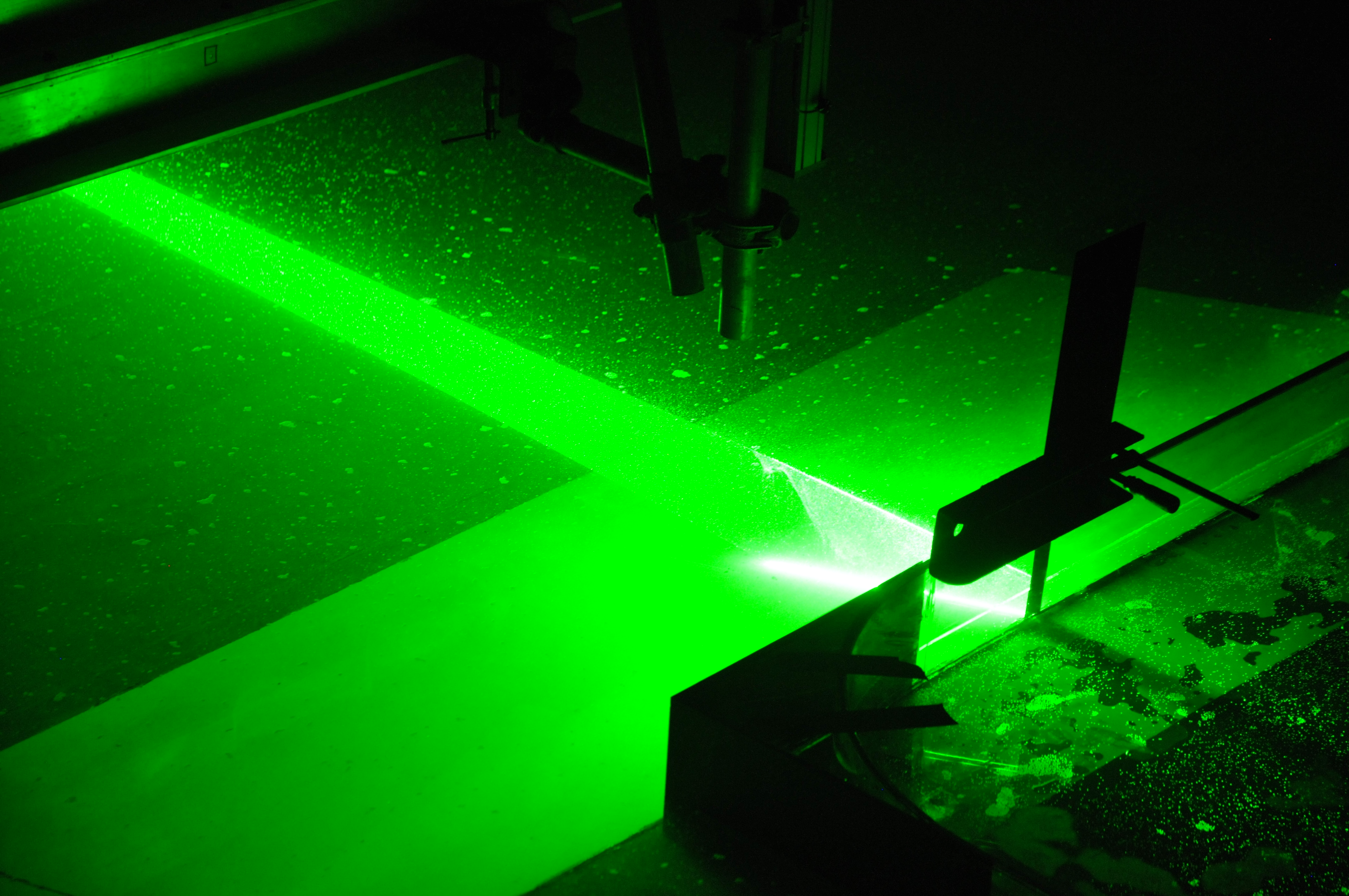
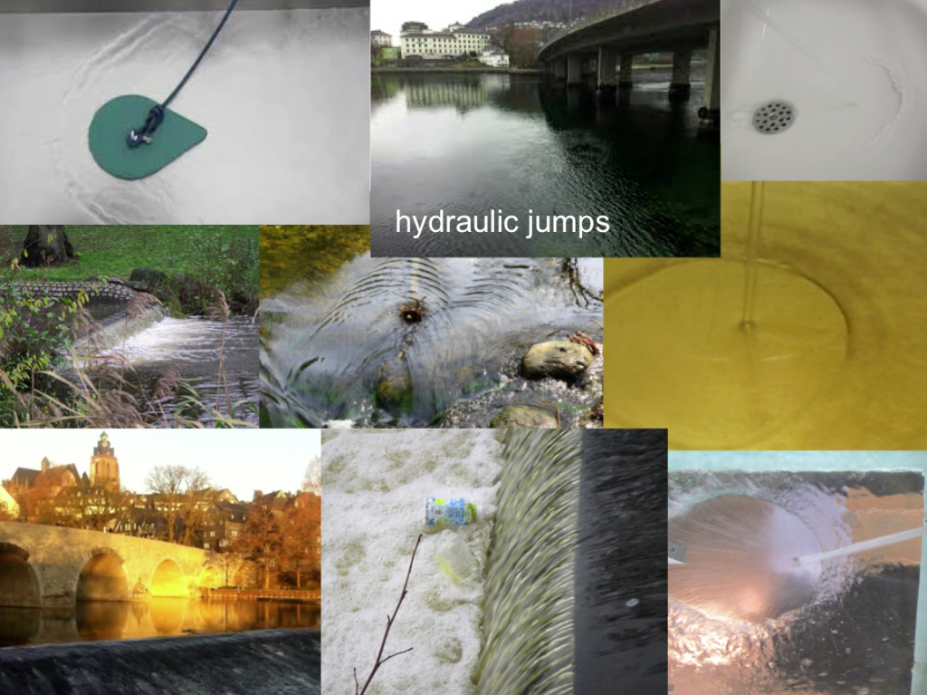
For a very strong example of where a Froude number helps you to describe a flow, look at the picture below: We use a hose to fill a tank. The water shoots away from the point of impact, flowing so much faster than waves can travel that the surface there is flat. This means that the Froude number, defined as flow velocity devided by phase velocity, is larger than 1 close to the point of impact.
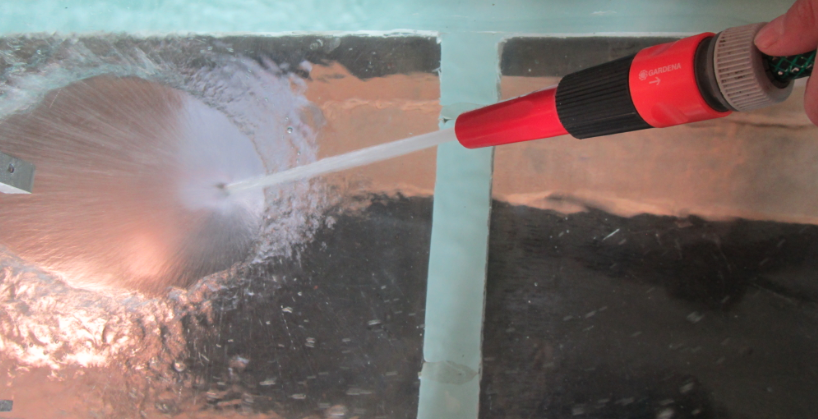
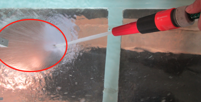
At some point away from the point of impact, you see the flow changing quite drastically: the water level is a lot higher all of a sudden, and you see waves and other disturbances on it. This is where the phase velocity of waves becomes faster than the flow velocity, so disturbances don’t just get flushed away with the flow, but can actually exist and propagate whichever way they want. That’s where the Froude number changes from larger than 1 to smaller than 1, in what is called a hydraulic jump. This line is marked in red below, where waves are trapped and you see a marked jump in surface height. Do you see how useful the Froude number is to describe the two regimes on either side of the hydraulic jump?
Obviously, this is a very extreme example. But you also see them out in nature everywhere. Can you spot some in the picture below?
But still, all those examples are a little more drastic than what we would imagine is happening in the ocean. But there is one little detail that we didn’t talk about yet: Until now we have looked at Froude numbers and waves at the surface of whatever water we looked at. But the same thing can also happen inside the water, if there is a density stratification and we look at waves on the interface between water of different densities. Waves running on a density interface, however, move much more slowly than those on a free surface. If you are interested, you can have a look at that phenomenon here. But with waves running a lot slower, it’s easy to imagine that there are places in the ocean where the currents are actually moving faster than the waves on a density interface, isn’t it?
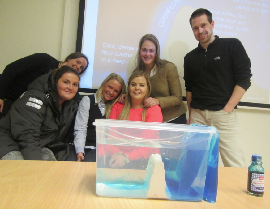
For an example of the explanatory power of the Froude number, you see a tank experiment we did a couple of years ago with Rolf Käse and Martin Vogt (link). There is actually a little too much going on in that tank for our purposes right now, but the ridge on the right can be interpreted as, for example, the Greenland-Scotland-Ridge, making the blue reservoir the deep waters of the Nordic Seas, and the blue water spilling over the ridge into the clear water the Denmark Strait Overflow. And in the tank you see that there is a laminar flow directly on top of the ridge and a little way down. And then, all of a sudden, the overflow plume starts mixing with the surrounding water in a turbulent flow. And the point in between those is the hydraulic jump, where the Froude number changes from below 1 to above 1.
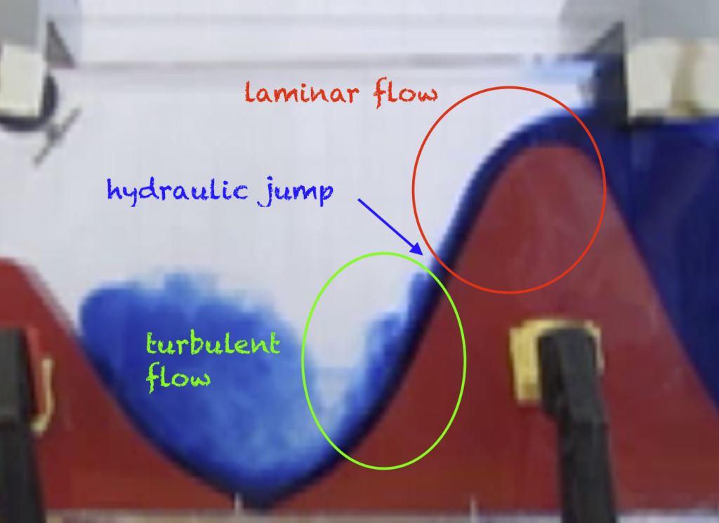
Nifty thing, this Froude number, isn’t it? And I hope you’ll start spotting hydraulic jumps every time you do the dishes or wash your hands now! :-)
When we come back from research cruises, one of the things that surprises people back home is how much time it takes to take measurements. And that’s for two reasons: Because the distances we have to travel to reach the area we are interested in are typically very large. And then because the ocean is also very deep.
People usually find it hard to imagine that it can easily take hours for an instrument, hanging on a wire from the ship, to go down all the way to the sea floor and then come back up to the ship again. A typical speed the winch is run at is 1 m/s. That means that for a typical ocean depth of 4 km, it takes 66 minutes for the instrument to go down, and then another hour to be brought back up to the ship. And then we haven’t even stopped the winch on the way up, which we usually do each time we want to take a water sample. So yes, the ocean is very deep!
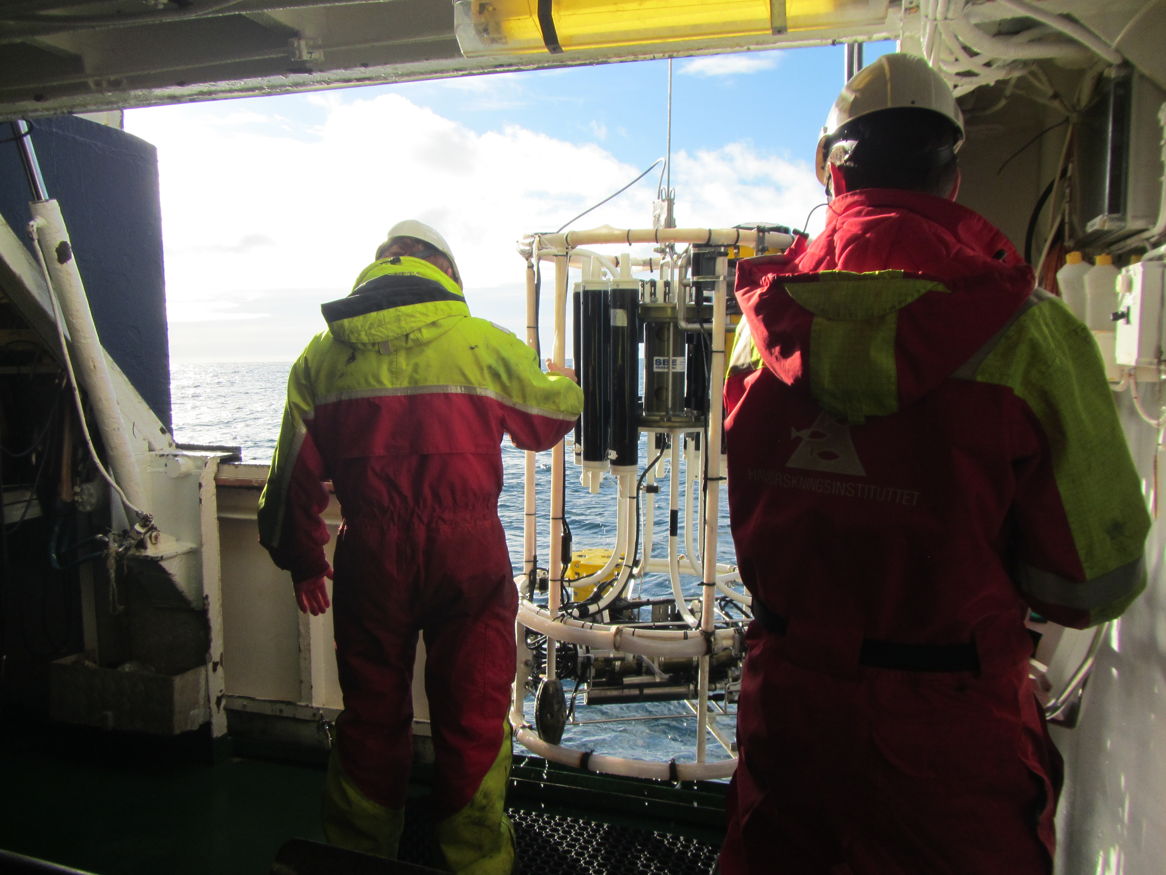
Jens and Arnt recovering the CTD
And yet, it is not deep. At least not compared to its horizontal extent. The fastest crossing of the Atlantic, some 5000km, took something like 3 days and 10 hours. And according to a quick google search, a container ship typically takes 10 to 20 days these days. So there is a lot of water between continents! And it is really difficult to imagine how large the oceans really are.
One way to describe the extent of the ocean is to use the L/H aspect ratio. It is just the ratio between a typical length (L), and a typical depth (H). A typical east-west length in the Atlantic are our 5000 km used above, and a typical depth are 4 km. This gives us an aspect ratio L/H of 5000/4 which is 1250. That is actually a really large aspect ratio — the horizontal length scales are a lot wider than the vertical ones.
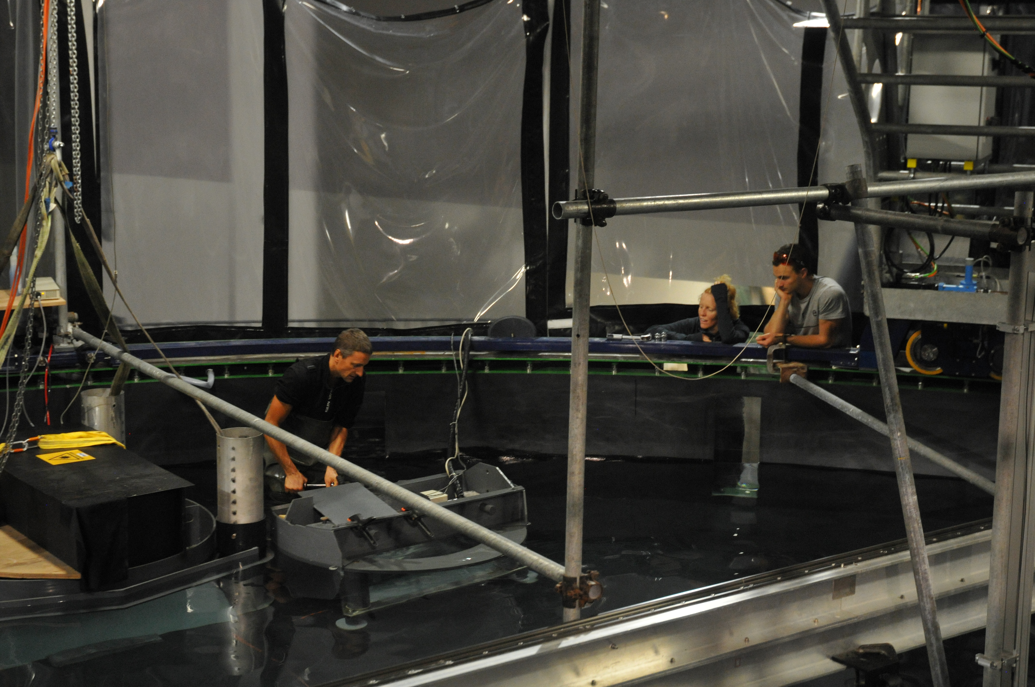
Now think about the kind of tank experiments we typically do. Here is a picture of a very simple Denmark Strait overflow experiment (more on that experiment here). You see the tank in the foreground, and a sketch of the same situation on the wall in the background. What you notice both for the experiment and the depiction is that in both cases the horizontal length scale is only about twice as much as the vertical one, leading to a L/H of 2.
Tank experiments at GFI
This L/H of 2, however, is supposed to represent a situation that in the real world has a horizontal scale of maybe 1000 km and a vertical one of maybe 1 km, which leads to a L/H of 1000. So you see that the way we typically depict sections through the ocean is very distorted from what they would look like if they were geometrically similar, meaning that they had the same L/H ratio, which means that they could be transformed into the real world just by uniformly stretching or shrinking.
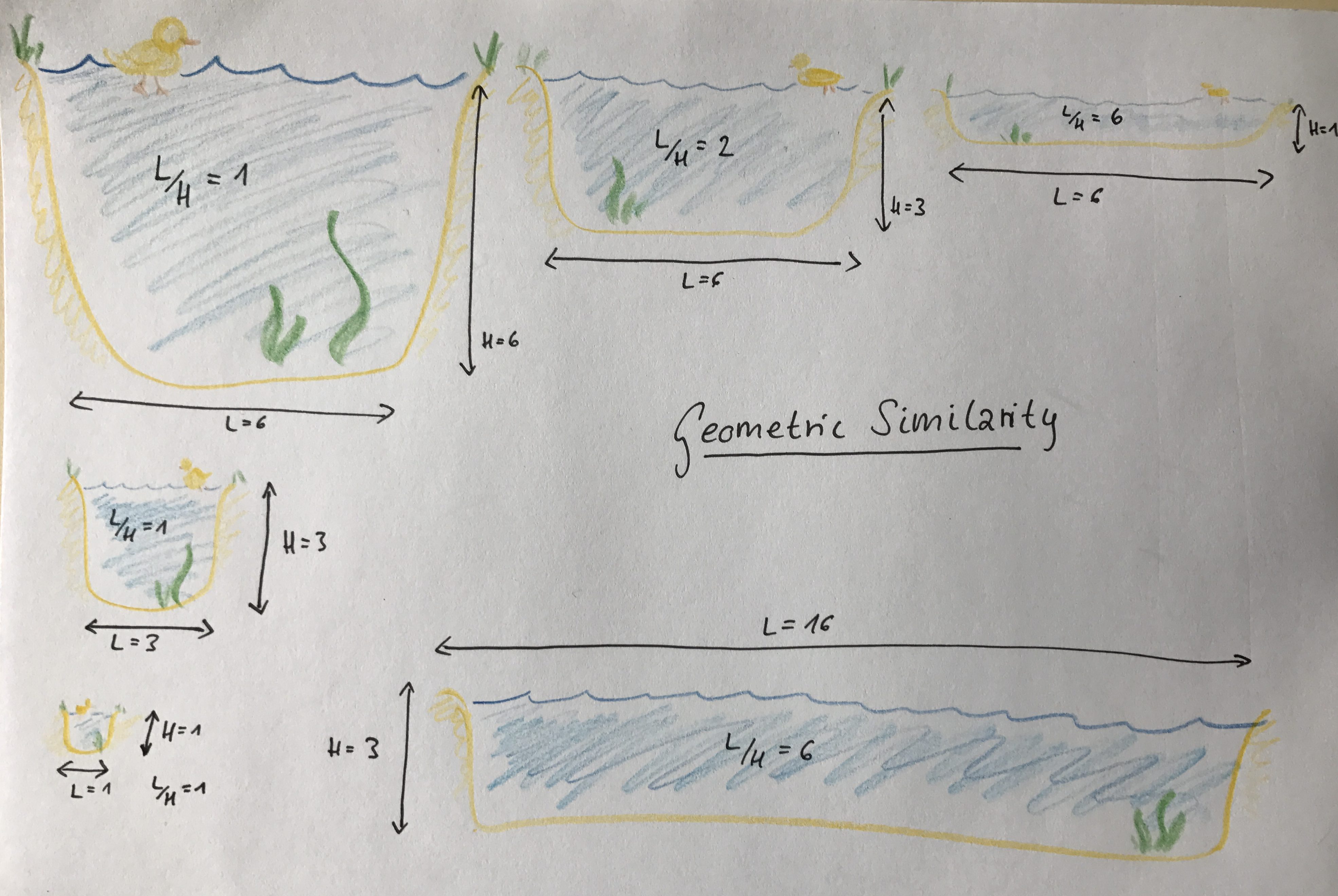
Below I have sketched a couple of duck ponds. The one on the left (with an aspect ratio L/H of 1) is geometrically shrunk below: Even though L and H become smaller, they do so at the same rate: their ratio stays the same. However going along the top row of duck ponds, the aspect ratio increases: While L stays the same, H shrinks. This means that the different ponds along the top of the picture are not geometrically similar. However, the one on the top right is geometrically similar to the one in the bottom right again (both have an L/H of 6). Does this make sense?
Sketch of different kinds of similarity
So in case you were wondering about why we need a tank that has 13 meters diameter — maybe now you see that it allows us to maintain geometric similarity a lot better than a smaller tank would, at least when we want to have water depths that are large enough that allow us to neglect surface tension effects and all that nasty stuff.
More on how Elin actually designed the experiments soon! :-)