Tag Archives: Coriolis platform

How the strength of the current influences which path it takes. First observations!

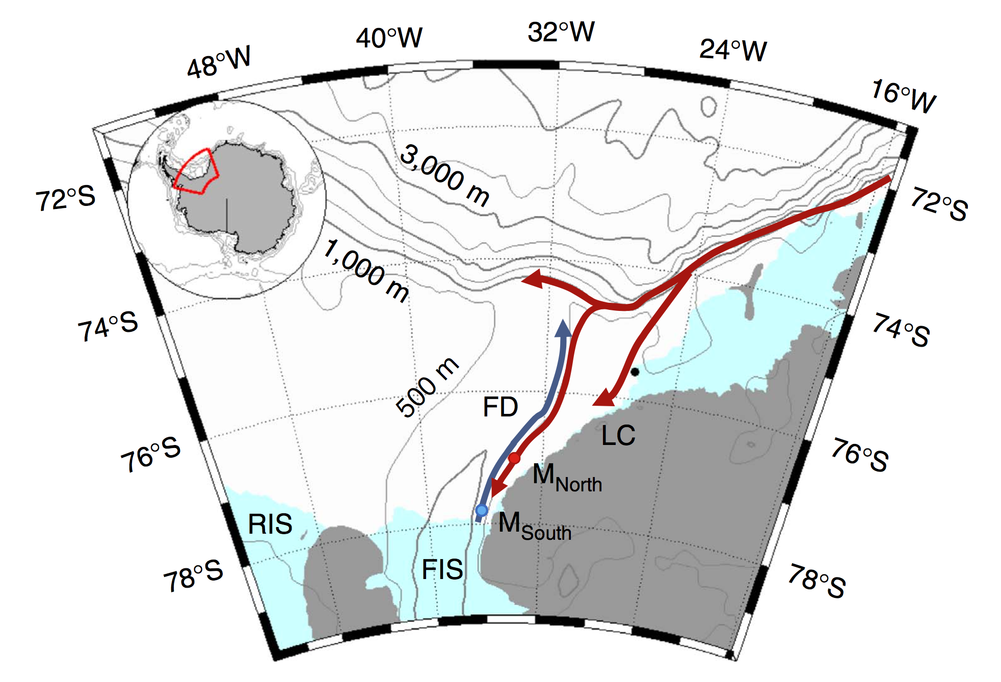
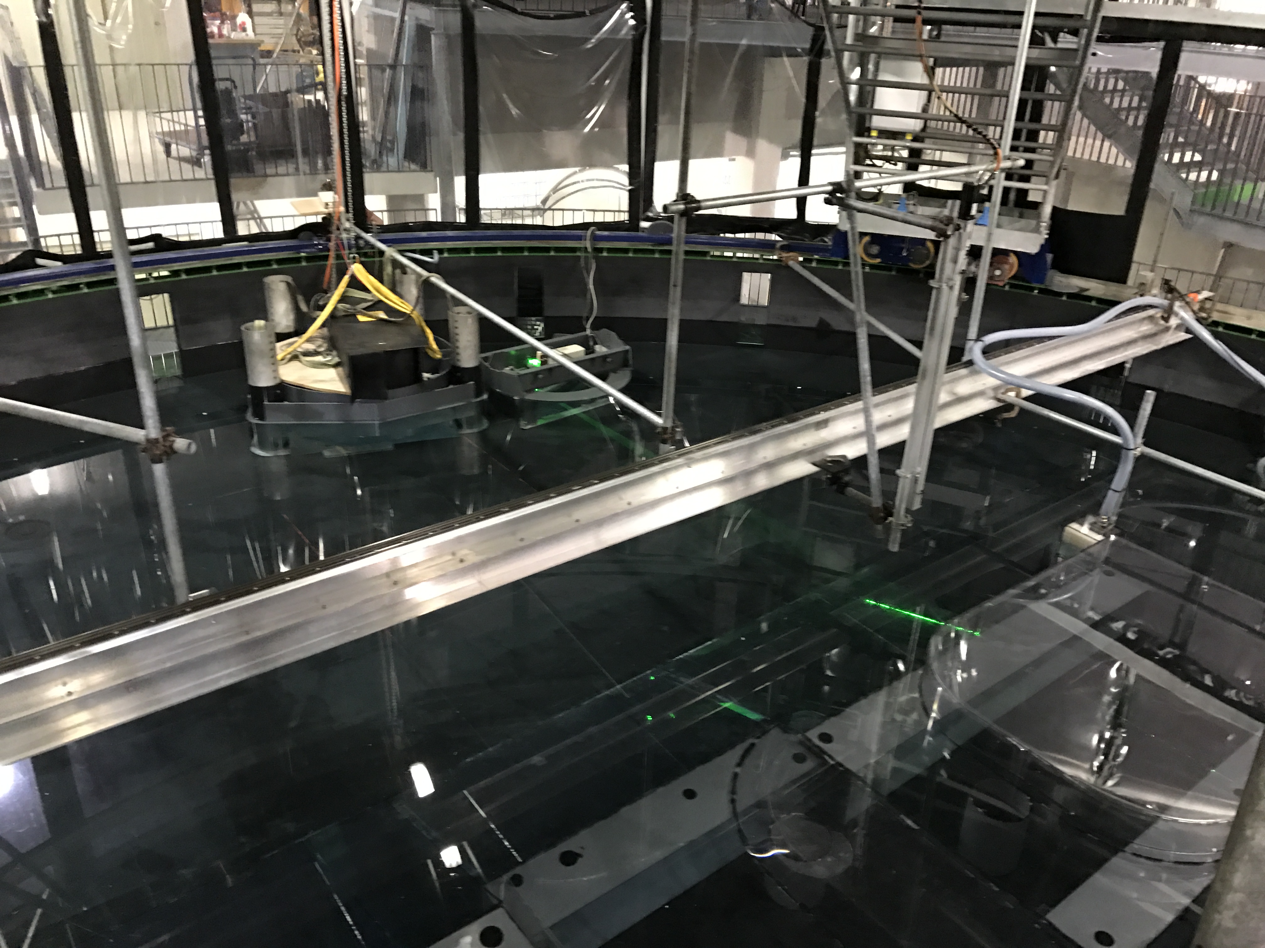
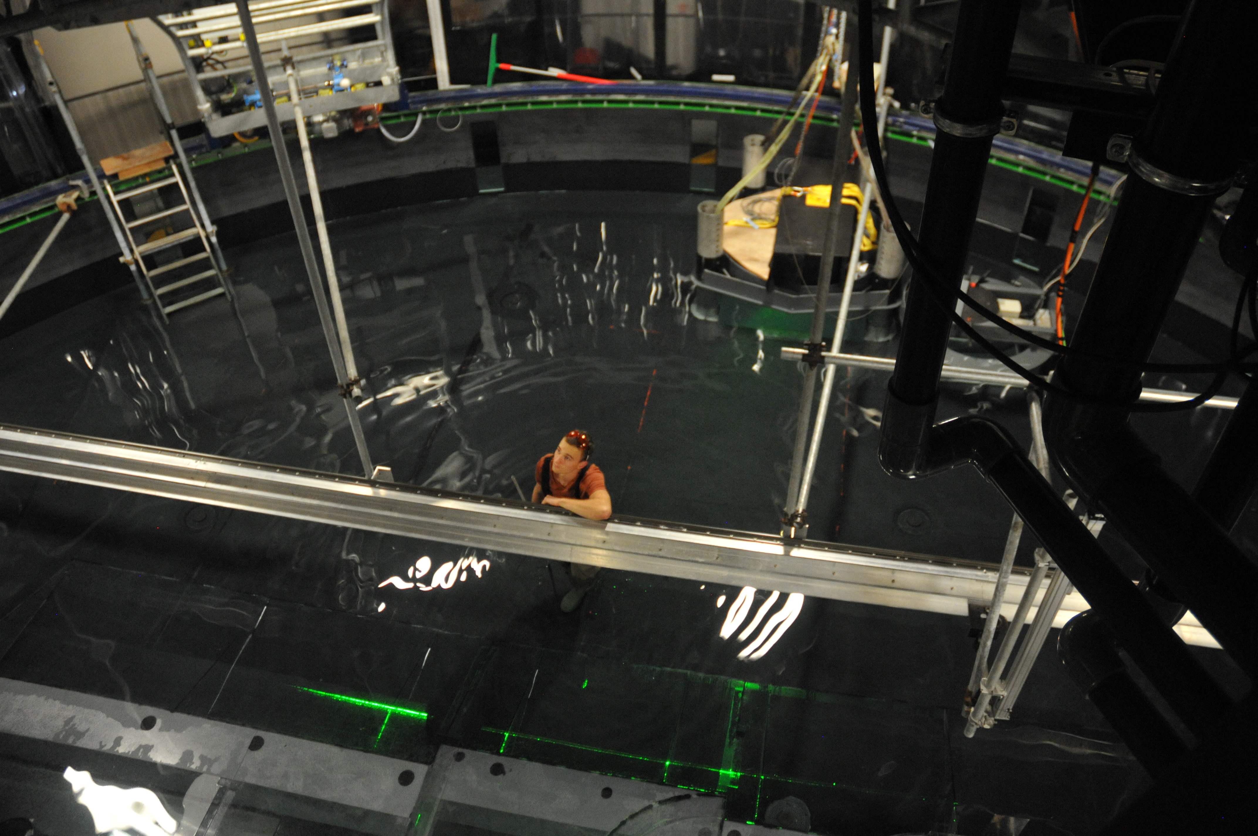
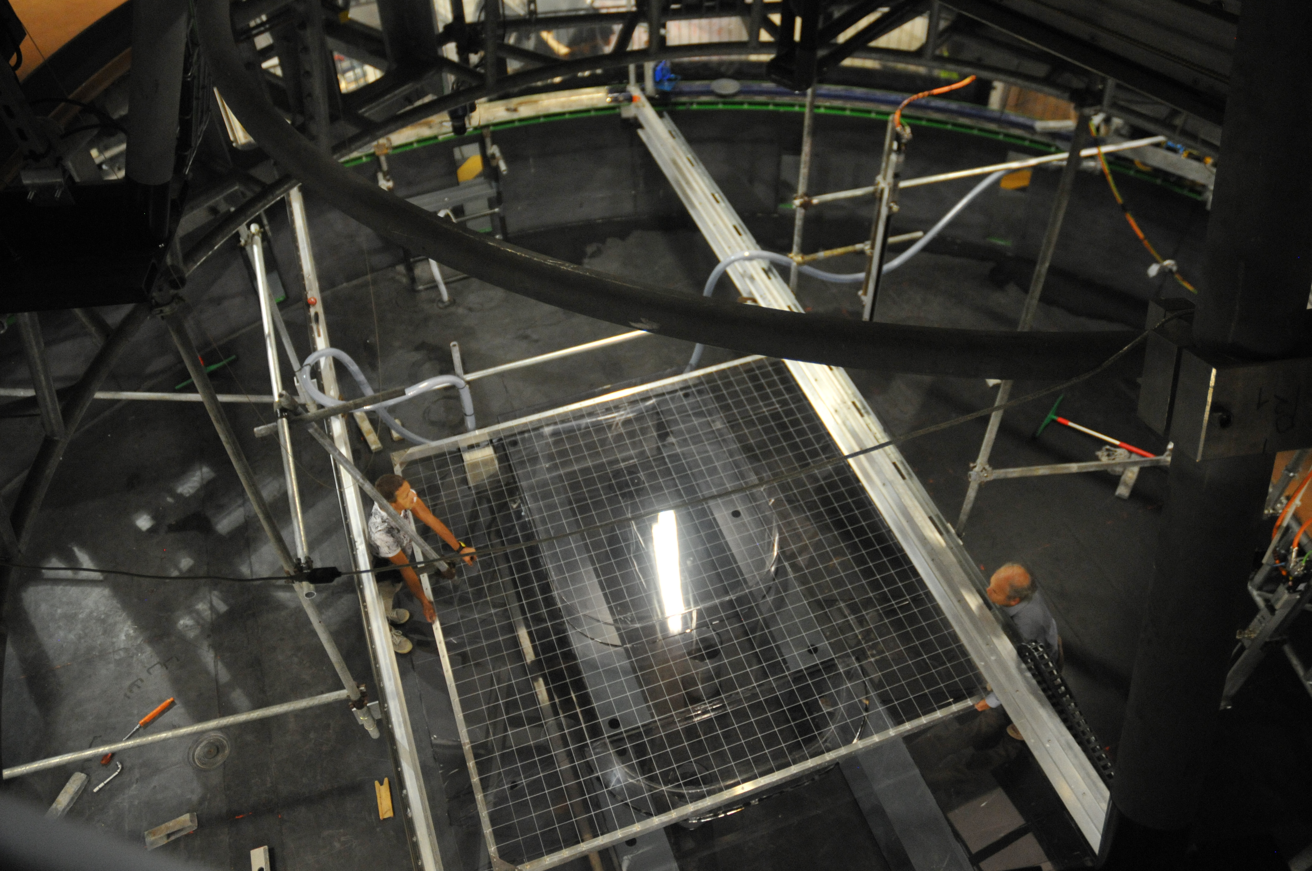
Depending on how strong a current we introduce in the 13-m-diameter rotating tank to simulate the strength of the coastal current in Elin et al.’s 2016 article (link on our blog, link to the article), it takes different pathway along and across our topography.

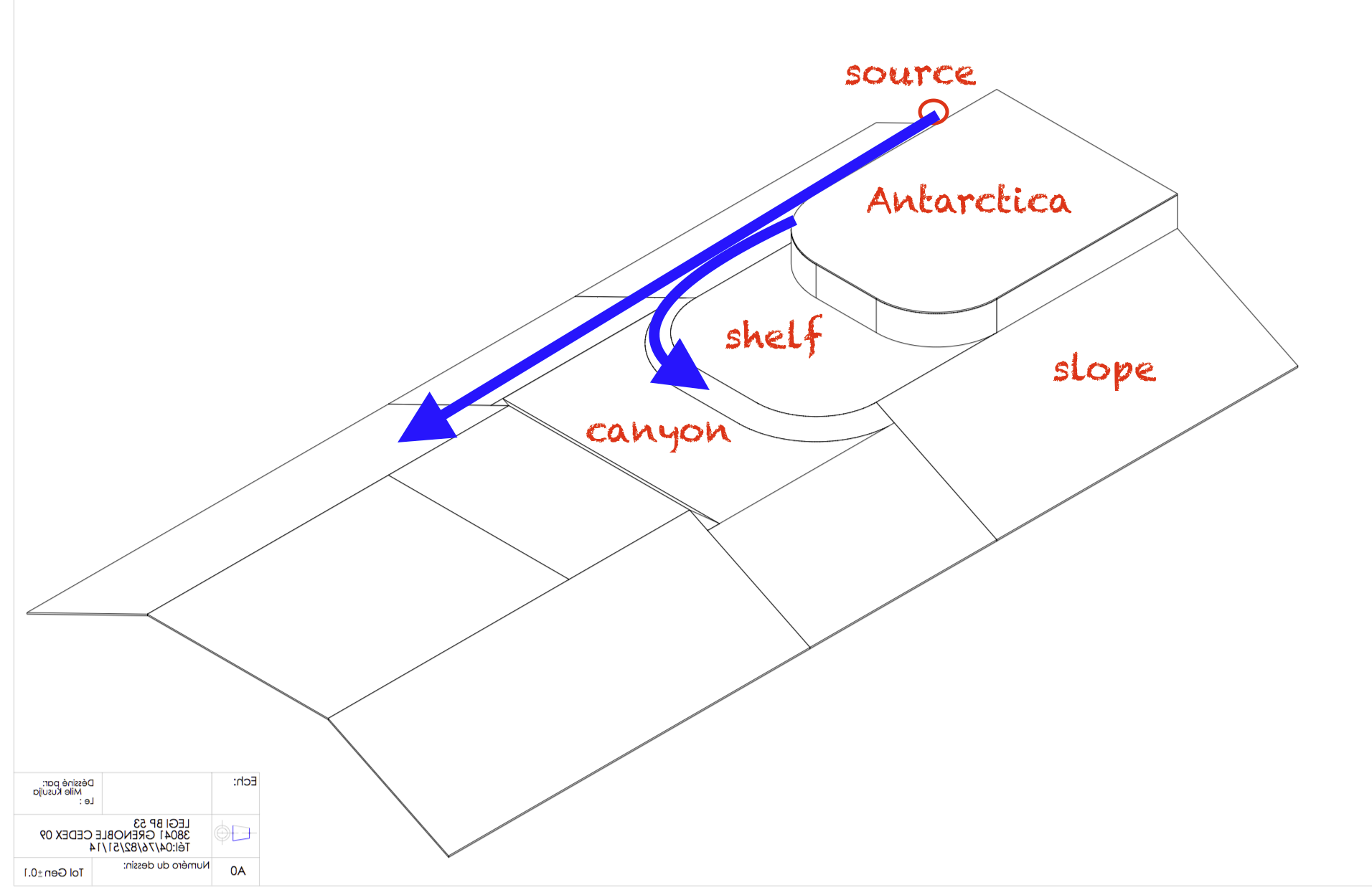
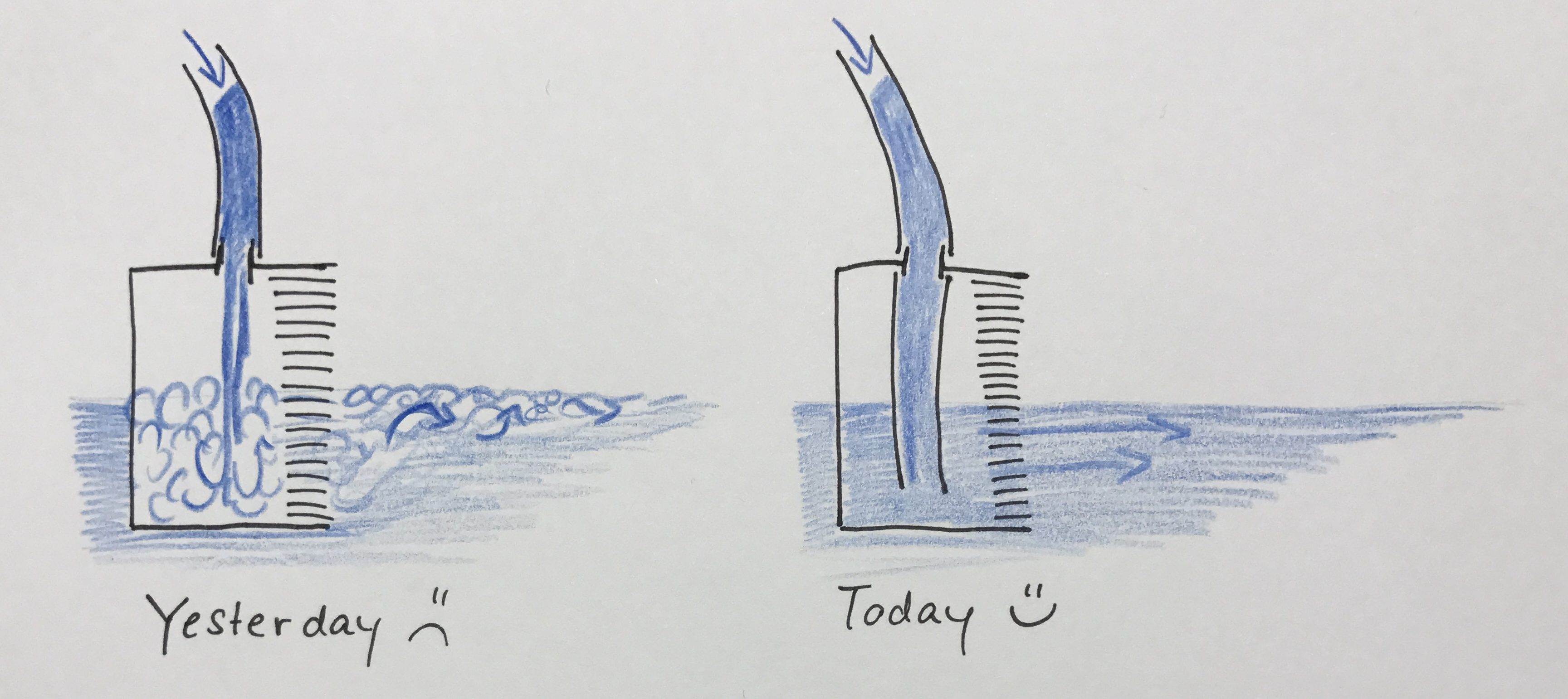
According to theory, we expected to see something like what I sketched below: The stronger the current, the more water should continue on straight ahead, ignoring the canyon that opens up perpendicular to the current’s path at some point. The weaker the current, the more should take a left into the canyon.

What we expect from theory

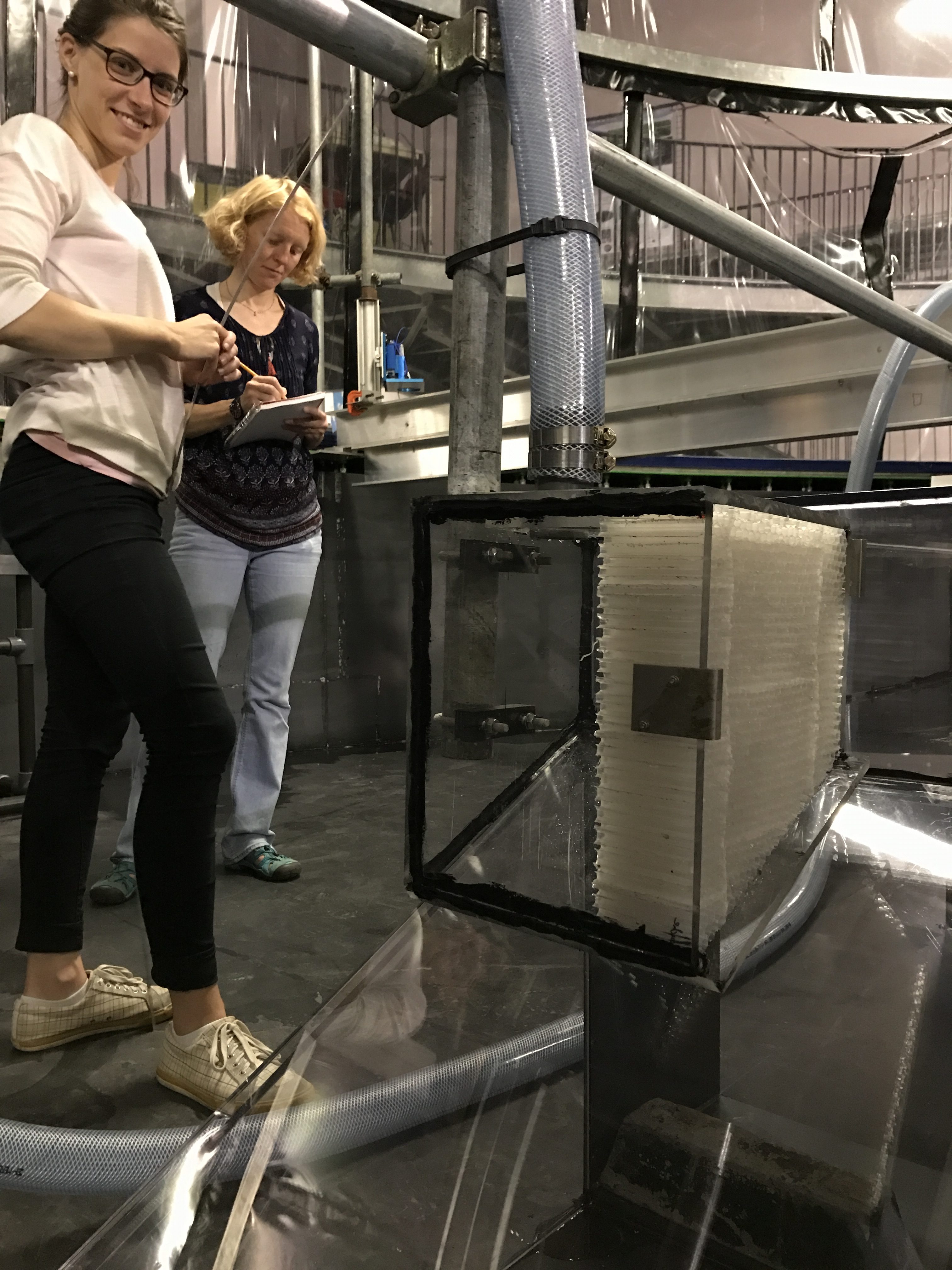
We have now done a couple of experiments, and here you get a sneak preview of our observations!

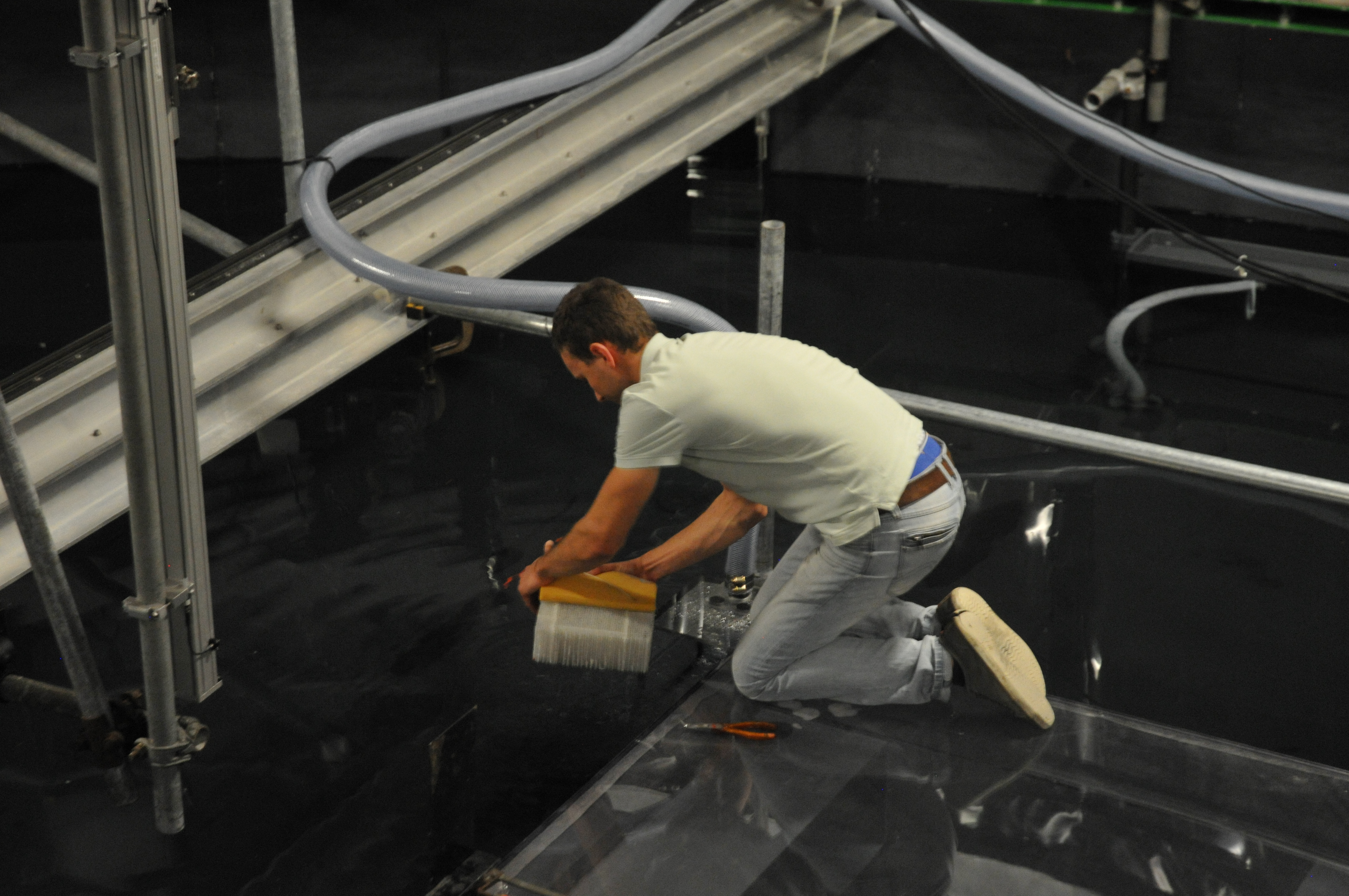
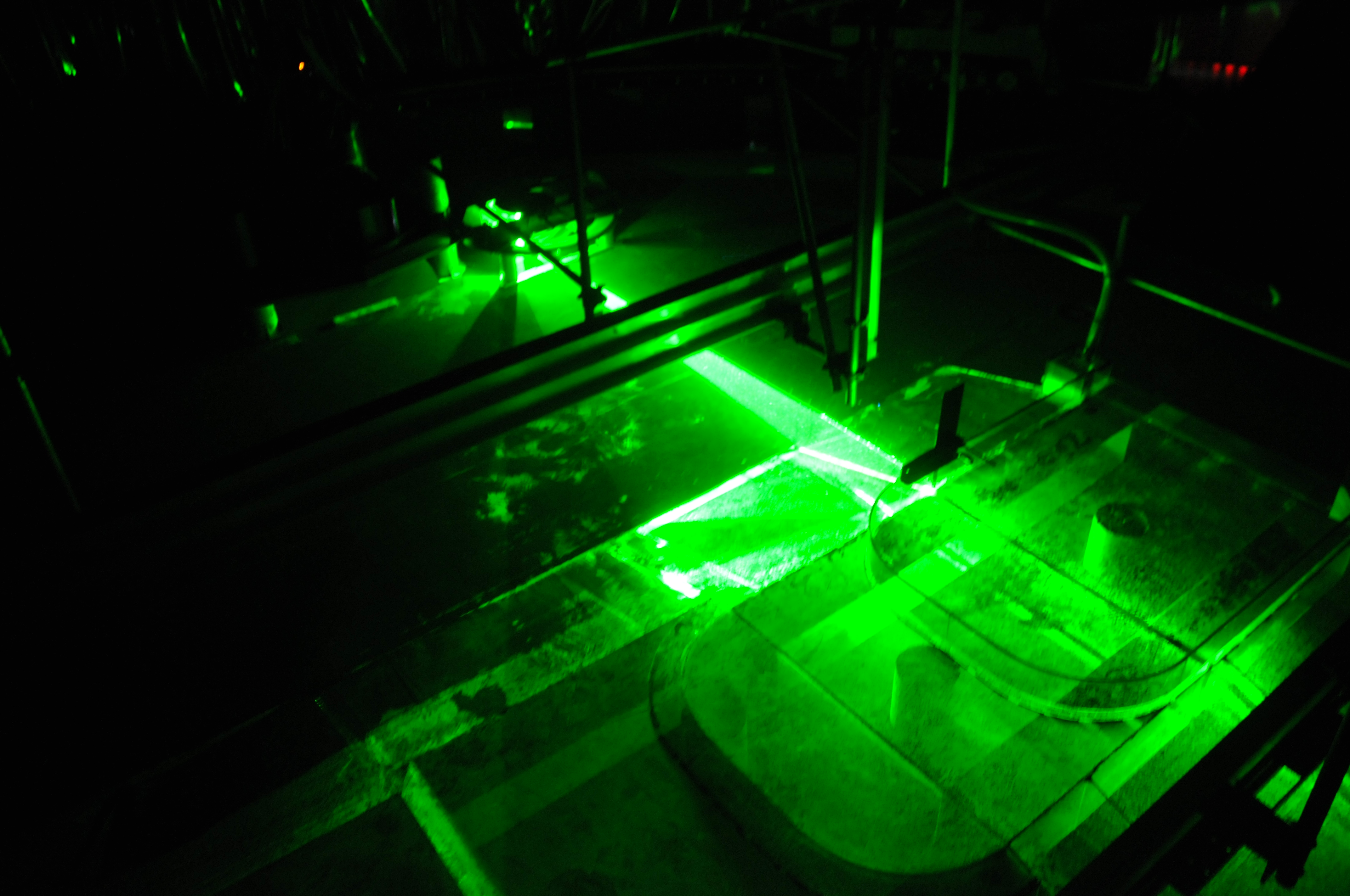
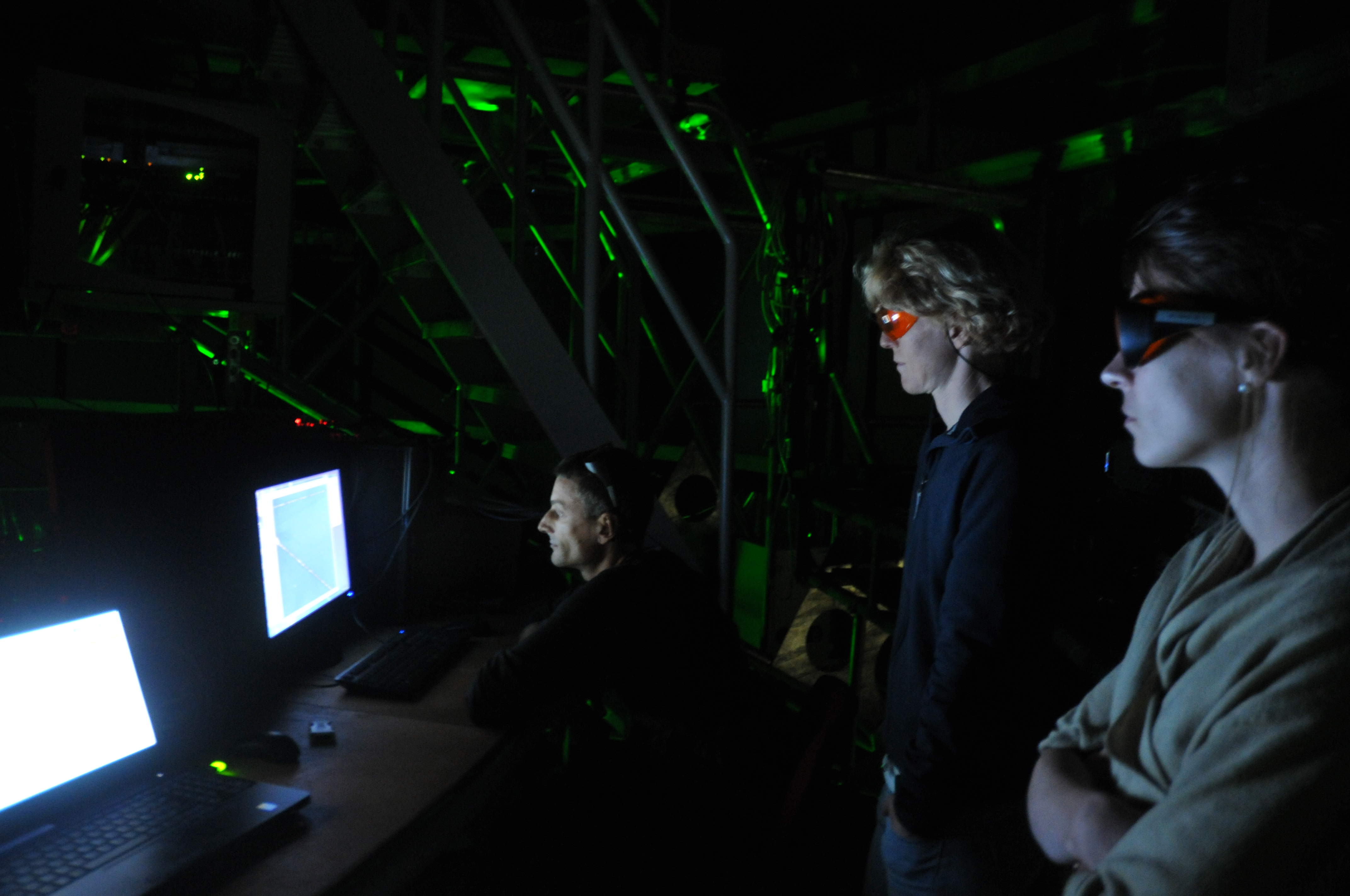
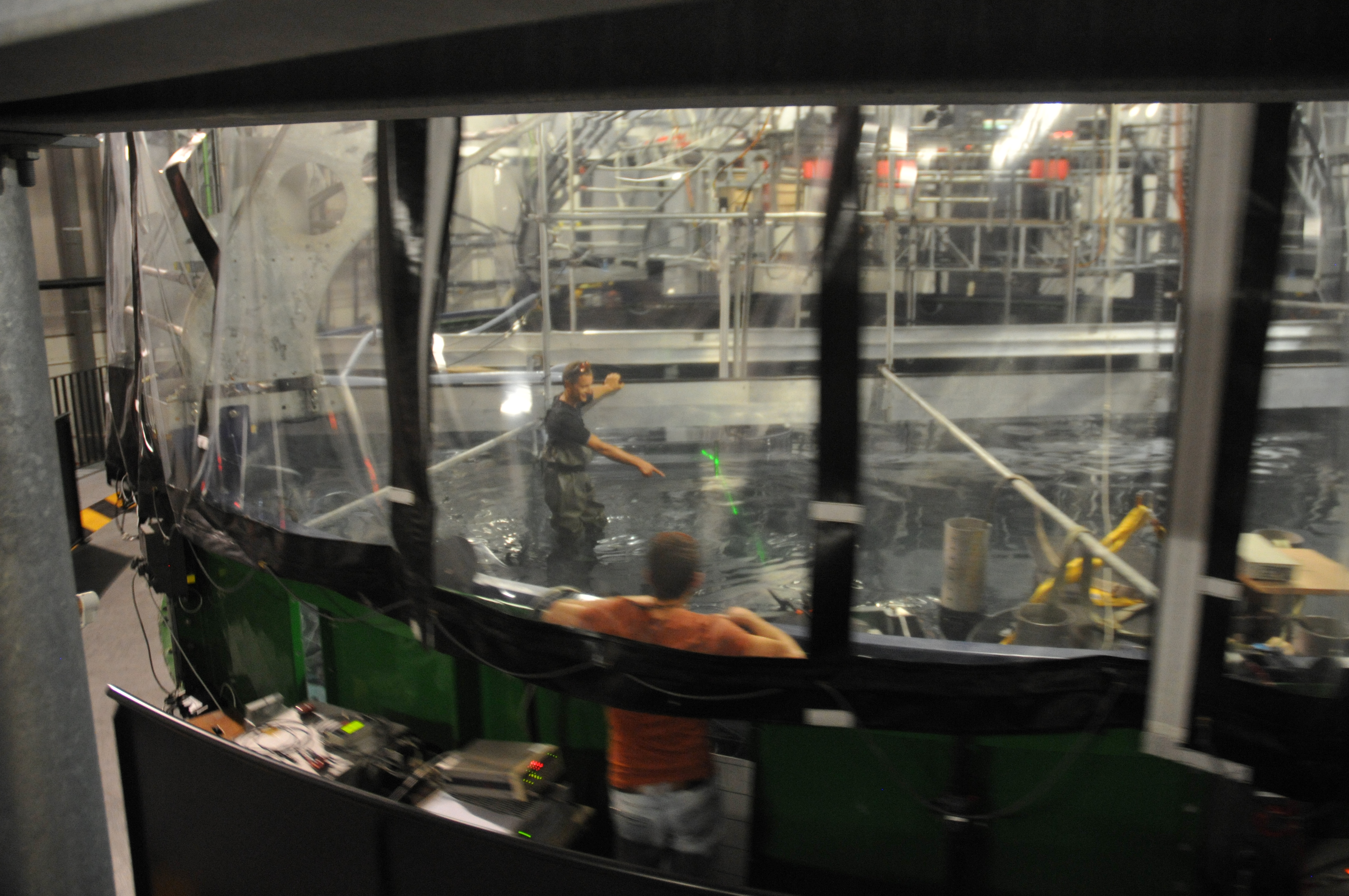
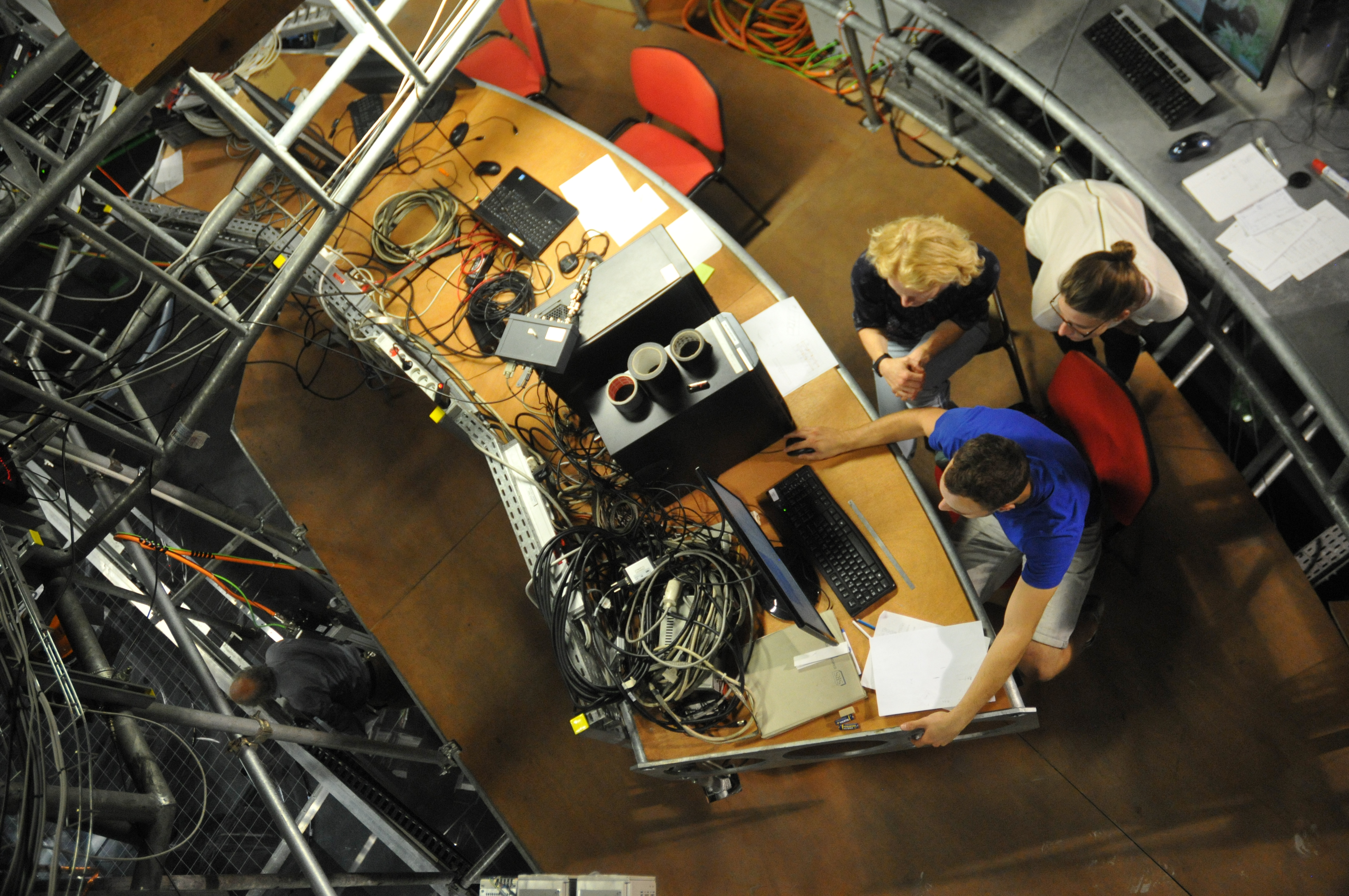
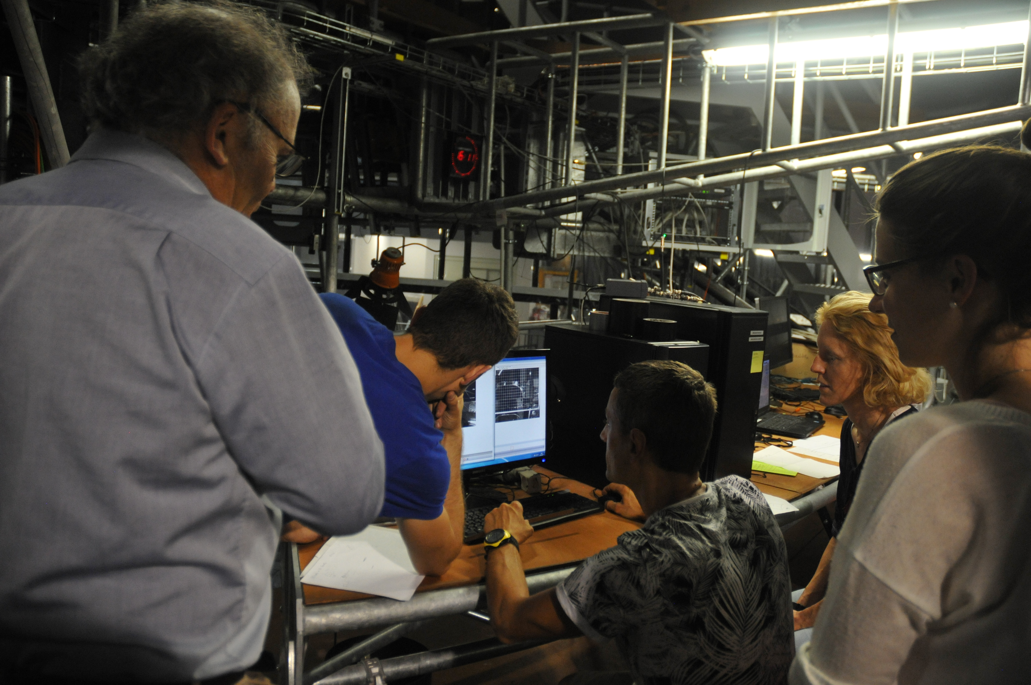
Small disclaimer beforehand: What you see below are pictures taken with my mobile phone, and the sketched pathways are what I have observed by eye. This is NOT how we actually produce our real data in our experiments: We are using cameras that are mounted in very precisely known positions, that have been calibrated (as described here) and that produce many pictures per second, that are painstakingly analysed with complex mathematics and lots of deep thought to actually understand the flow field. People (hi, Lucie!) are going to do their PhDs on these experiments, and I am really interpreting on the fly while we are running experiments. Also we see snapshots of particle distribution, and we are injecting new particles in the same tank for every experiment and haven’t mixed them up in between, so parts of what you see might also be remnants of previous experiments. So please don’t over-interpret! :-)

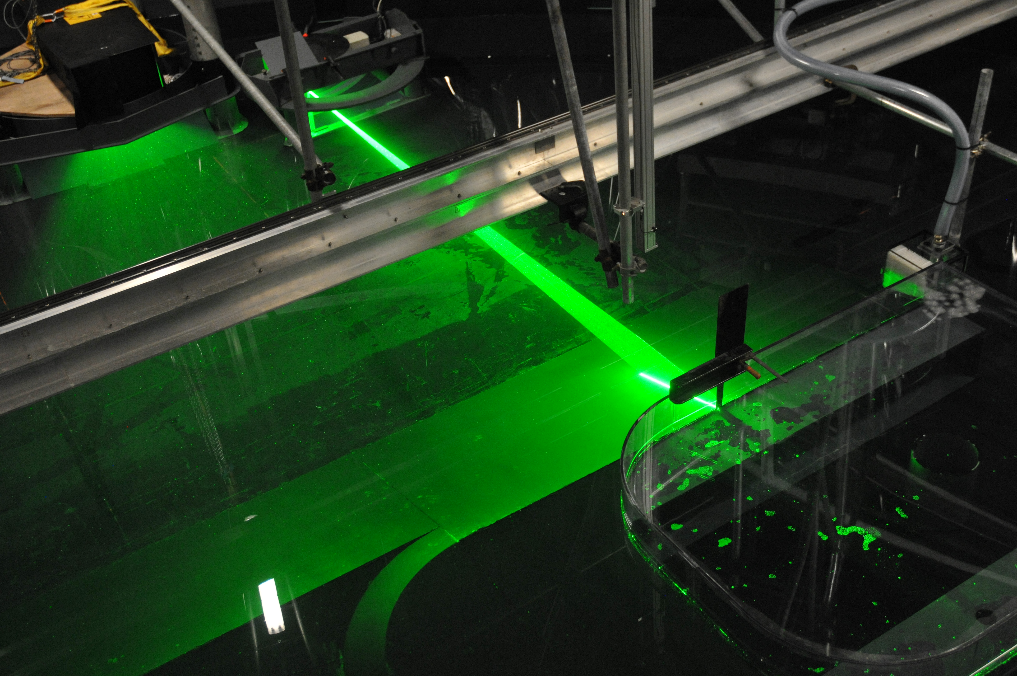
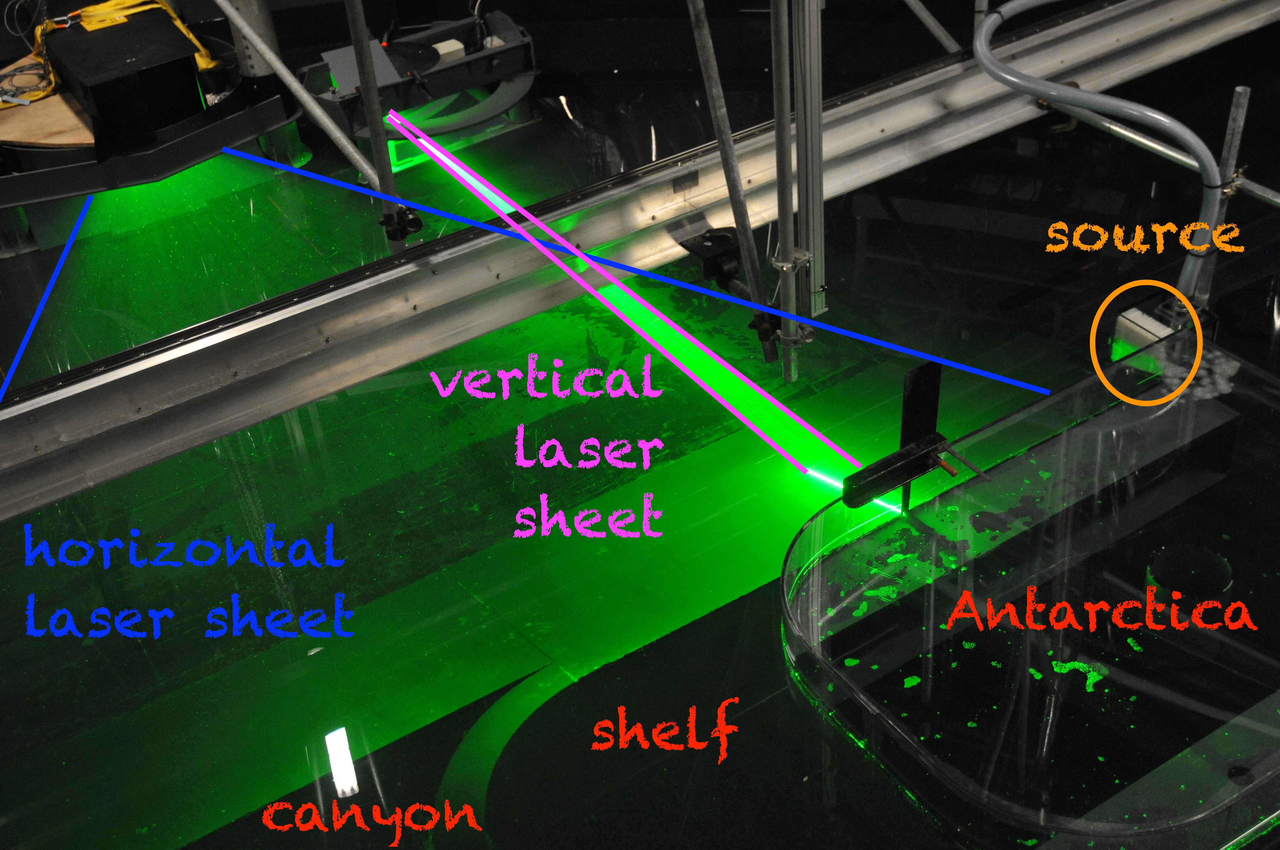
So here we go: For a flow rate of 10 liter per minute (which is the lowest flow rate we are planning on doing) we find that a lot of the water is going straight ahead, while another part of the current is following the shelf break into the canyon.

First observations – low flow rate (10l/min)

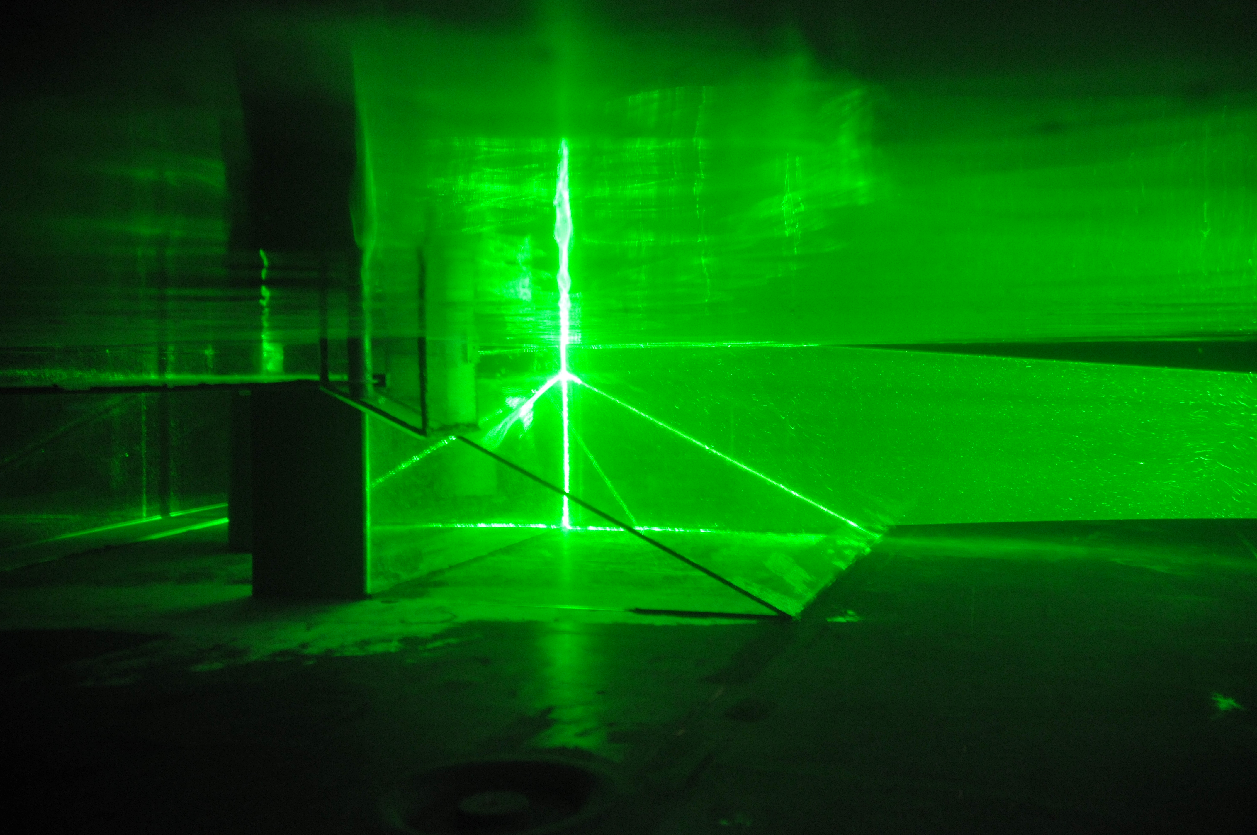
For 20 liter per minute, our second lowest flow rate, we find that parts of the current is going straight ahead, parts of it is turning into the canyon, and a small part is following along the coastline (Which we didn’t expect to happen). However it is very difficult to observe what happens when the flow is in a steady state, especially when velocities are low, since what jumps at you is the particle distribution that is not directly related to the strength of the current which we are ultimately interested in… So this might well be an effect of just having switched on the source and the system still trying to find its steady state.

First observations – higher flow rate (20l/min)

The more experiments we run in a day after only stirring the particles up in the morning, the more difficult it gets to observe “by eye” what is actually happening with the flow. But that’s what will be analysed in the months and years to come, so maybe it’s good that I can’t give away too many exciting results here just yet? ;-)

How our experiments relate to the real Antarctica

Leave a reply

After seeing so many nice pictures of our topography and the glowing bright green current field around it in the tank, let’s go back to the basics today and talk about how this relates to reality outside of our rotating tank.

Figure 1 or Darelius, Fer & Nicholls (2016): Map. Location map shows the moorings (coloured dots), Halley station (black, 75°350 S, 26°340 W), bathymetry and the circulation in the area: the blue arrow indicates the flow of cold ISW towards the Filchner sill and the red arrows the path of the coastal/slope front current. The indicated place names are: Filchner Depression (FD), Filchner Ice Shelf (FIS), Luipold coast (LC) and Ronne Ice Shelf (RIS).

Above you see the red arrows indicating the coastal/slope front currents. Where the current begins in the top right, we have placed our “source” in our experiments. And the three arms the current splits into are the three arms we also see in our experiments: One turning after reaching the first corner and crossing the shelf, one turning at the second corner and entering the canyon, and a third continuing straight ahead. And we are trying to investigate which pathway is taken depending on a couple of different parameters.

The reason why we are interested in this specific setup is that the warm water, if it turns around the corner and flows into the canyon, is reaching the Filchner Ice Shelf. The more warm water reaches the ice shelf, the faster it will melt, contributing to sea level rise, which will in turn increase melt rates.

In her recent article (Darelius, Fer & Nicholls, 2016), Elin discusses observations from that area that show that pulses of warm water have indeed reached far as far south as the ice front into the Filchner Depression (our canyon). In the observations, the strength of that current is directly linked to the strength of the wind-driven coastal current (the strength of our source). So future changes in wind forcing (for example because a decreased sea ice cover means that there are larger areas where momentum can be transferred into the surface ocean) can have a large effect on melt rates of the Filchner Ice Shelf, which might introduce a lot of fresh water in an area where Antarctic Bottom Waters are formed, influencing the properties of the water masses formed in the area and hence potentially large-scale ocean circulation and climate.

The challenge is that there are only very few actual observations of the area. Especially during winter, it’s hard to go there with research ships. Satellite observations of the sea surface require the sea surface to be visible — so ice and cloud free, which is also not happening a lot in the area. Moorings give great time series, but only of a single point in the ocean. So there is still a lot of uncertainty connected to what is actually going on in the ocean. And since there are so few observations, even though numerical models can produce a very detailed image of the area, it is very difficult how well their estimates actually are. So this is where our tank experiments come in: Even though they are idealised (the shape of the topography looks nothing like “real” Antarctica etc.), we can measure precisely how currents behave under those circumstances, and that we can use to discuss observations and model results against.

—

Darelius, E., Fer, I., & Nicholls, K. W. (2016). Observed vulnerability of Filchner-Ronne Ice Shelf to wind-driven inflow of warm deep water. Nature communications, 7, 12300.

Water jet pumps, and why we don’t like them in our experiments

Leave a reply

Just a quick update from the lab tonight: We are fixing more bugs by the hour :-)

First: the bubble-free source.

I have previously written about how we thought we were going to get our source bubble-free (link here). Turns out, it’s not quite as easy as we thought — there were still plenty of bubbles everywhere! But luckily, Thomas came to our rescue and put some foam inside the source so the water has to pass through there before leaving the source through the honeycomb. That effectively gets rid of all the bubbles since they just don’t fit through and surface inside the source box instead of outside of it in our experiment. We were really concerned about all those bubbles for two reasons: A) They might show up in the pictures we want to analyse and destroy any correlations we are hoping to find since they are there one second and then burst and disappear the next. And B) since the bubbles left the source below water level, they popped up to the surface and introduced vertical flow where we really didn’t want it.

But anyway, the bubbles are gone now! It’s amazing how well that works and all our (ok, my) prophecies of doom (the water is never to go through the foam! It is going over it and then enter the tank as a water fall! And even if it does go through, the particles we need to visualize the flow with, won’t!) were completely unnecessary.

Thomas kneeling on Antarctica, fixing the source

Second: The unwanted water jet pump.

We don’t actually know where it happened, but somewhere there was a leak and air got pulled into our inflow. Thomas and Samuel fixed this problem, too, but this is what happened: We have quite a fast flow from a reservoir sitting high above the tank down to the source. The faster the flow, the lower the pressure in it, which means that it sucks stuff (in our case air) from the surroundings, and entrains it. And that’s exactly the effect that is used in water jet pumps, except there people want it to happen…

Below you see an example of the Isère here in Grenoble, where a rather fast flow is causing a return flow as soon as the river bed widens a little.

Sketch of how a water jet pump works, using the Isere as example

Anyway, now it’s almost dinner time in our shared flat. But we’ll be back tomorrow with first results from our experiments! :-)

What are we actually trying to measure in our rotating swimming pool?

Leave a reply

You’ve heard us talk a lot about rotating swimming pools. Nadine has written about why we care about Antarctic ice shelf melting (link), why the ice shelf is melting (link) and how we are going to investigate it (link). Today, I am going to bring those explanations together with all that you’ve seen so far about our experiments in Grenoble. I hope! :-)

Let’s start with a technical drawing of our “Antarctica”, the topography we have in the middle of the tank. You have seen it in many of our previous posts: It’s the thing that used to be in clear plastic, but that one early morning got painted black.

Sketch of our topography and what currents we expect to see in our experiment

What we are going to investigate is how a current, introduced at the “source”, will behave. We expect that it will flow along the shelf break and that some of it will flow around the corner into the canyon, while some of it will continue on straight ahead. How large a portion of the current takes which part depends on several parameters, which we will systematically change over the next couple of weeks: How large the source’s flow rate is (we are starting with 50 liter per minute), whether there is a density difference between the source water and the ambient water (we are starting with no density difference) and what happens if we add a sharp corner to the nice and smooth corner of Antarctica and the shelf.

So far, so good. When we look down from the rotating first-floor office, things look a little different (an annotated version further down this page):

Woah! It is happening! Laser sheets and currents are on!

You see (parts of) the topography in the lower right corner of the image. And then you see a lot of green light: Our laser sheets! The laser sheets will illuminate thin layers of water, which we can take pictures of with cameras mounted perpendicularly to the sheets. That in itself isn’t so exciting, but we will have neutrally buoyant particles in the water, which light up when lit with the laser. If we take enough pictures of the particles, we can track individual particles as they get advected by the currents, and thus get a good idea of the flow field that is illuminated by the lasers.

Details of the experimental setup: Position of laser sheets, source, topography

And the cool thing is that we have not only one, but six vertical laser sheets, that are used sequentially. Below you see our first experiment and each picture in the animated gif is showing you a different layer, so you get an idea of the vertical shape of the flow field.

And these are the first current fields we are observing!

Isn’t this amazing? How lucky are we that we got the opportunity to travel to Grenoble to see all this? :-)

Getting rid of bubbles in our jet

Leave a reply

Sometimes the devil is in the details…

On our first day at the Coriolis platform in Grenoble, I took a picture of the “source” in our experiments (see above): The plastic box that is fed by a hose from above and that has one open side with a “honeycomb” (or: a make-the-outflowing-water-nice-and-laminar thingy, technical term) that introduces the water into the tank that we want to follow around Antarctica.

This source is sitting against our topography, and will be partly submerged so that we introduce the jet at water level and below (instead of having a waterfall going in). The idea is to get a nice and bubble-free flow because — as we talked about yesterday — bubbles reflect the laser very strongly and disguise the signal that we are actually interested in.

So when we were doing our first tests last night, the first step was to flush out all the bubbles from all the pipes and hoses that supply the water to our source. Except that bubbles kept coming. And coming. Until, at some point, we realised that this was the problem:

Sketch of “the bubble issue”

The inflowing water was free-falling through air before hitting the water inside the source box, thus entraining a lot of air bubbles directly inside of the source. Good luck flushing them out… The solution was to add an extra piece of hose to just below the water surface so no air can be entrained.

So when we arrived at the lab this morning to an empty tank* we were delighted to see that the amazing Samuel and Thomas had already fixed the source!

“Antarctica” in the tank which is empty yet again…

*Yes, the tank really was empty again. Turns out that the reflection of the laser off the topography is so strong that it’s both a problem for data quality and that too much of the light gets scattered out of the water to be safe when we use the laser at it’s real setting for the experiments rather than at the super low setting we used for the tests… Disappointing, yes, but we were so surprised and pleased when we arrived this morning and the topography had already been painted AND the source been fixed! We are super impressed with and grateful to the awesome team here in Grenoble! :-) And we are happy to report that there is water in the tank again and we can start measuring after lunch!

We have water in our rotating tank! Now testing the lasers

Leave a reply

Above you see the very first water coming into our tank. Only a couple of hours, and the tank was full! And in solid body rotation (since it has been spinning all the time while being filled) which means that we can start doing the real experiments very soon! :-)

Most of the afternoon has been spent testing the lasers that will be used later to measure flow velocities inside the water around our topography. Laser testing isn’t something where we can help with, but that doesn’t keep us from having fun with safety goggles! Although it took us a little while to figure out that while the goggles made the laser invisible (or, hopefully, blocked it from coming anywhere near our eyes) we could see on the displays of our cameras whether the laser was on or off!

Safety first! Fancy goggles protecting Mirjam, Elin and Nadine’s eyes from the lasers

Below you see the laser going through the water and illuminating the topography in the lower right corner of the image.

Green laser beams in the water!

What needed to be done then was to make sure that the laser sheet is actually at exactly the position we want it to be.

When you look in from the side through the water, you see the shape of our topography illuminated and the vertical laser sheet coming in from the right.

Green laser beams in the water, reflecting off of our topography

Same if you look in from the top: Do you recognise our little Antarctica? Below we see a vertical laser sheet.

Green laser beams in the water, illuminating “Antarctica”

What the “official” camera sees can be observed on a screen in our second-floor office:

Checking out the recordings from the second floor (co-rotating) office

And what we saw is that there are way too many bubbles on the topography still, that show up as bright spots (which distract from the particles that we specifically seed to visualize currents). So: Someone needed to go in and clean…

Samuel cleaning bubbles off the topography so they don’t distort the laser beam

We could observe on the screen how the bubbles were swept away!

Bubble-sweeping being observed on the screen

Next, it was time to set the exact positions we want the laser sheets at.

Nadine helps Samuel program the laser sheets to the perfect positions

For the horizontal sheets, this is done by having someone stand in the tank and actually measure the height at which the laser hits a ruler for a given setting.

Thomas measuring the height of the laser sheets in the tank

But now I am going to pick up Lucie, or new team member, at the tram stop and hope that we are ready to start the real experiments first thing tomorrow morning! :-)

Why do we go to all the hassle of rotating our swimming pool?

Leave a reply

This blog post was written for Elin Darelius & team’s blog (link) which you should totally follow if you aren’t already!

—

We have started rotating and filling water into our 13-meter-diameter rotating tank! So exciting! Pictures of that to come very soon.

But first things first: Why do we go to the trouble of rotating the swimming pool?

The Earth’s rotation is the reason why movement that should just go straight forward (as we learned in physics class) sometimes seems to be deflected to the side. For example, trade winds should be going directly towards the equator from both north and south, since they are driven by hot air rising at the equator, which they are replacing. Yet we see that they blow towards the west in addition to equatorward. And that is because the Earth is rotating: So even though the air itself is only moving towards the equator, when observed from the Earth, the winds seem to be deflected by what is called the Coriolis force.

The influence of the Coriolis force becomes visible when you look at weather systems, which also swirl, rather than air flowing straight to the center where it then raises. Or when you look at tidal waves that propagate along a coastline rather than just spreading out in all directions. Or when you look at ocean currents. But all of these effects are fairly large-scale and not so easy to observe directly by just looking up in the sky or out on the ocean for a short while.

There are however easy ways to experience the Coriolis force when you play on a merry-go-round or with a record player or with anything rotating, really. Those are obviously spinning much faster than the Earth, and that’s exactly the point: The faster rotation makes it easy for us to see that something is going on. And obviously, Nadine and I had to test just that on the best merry-go-round that I have ever seen:

And that is what we’ll use in our experiments, too: Since our topography is a lot smaller than the real world it is representing, we also have to turn the tank faster than the real world is turning in order to get comparable flow fields. How to exactly calculate how fast we need to turn we’ll talk about soon. Stay tuned! :-)

Nadine demonstrating the — southern hemisphere! — Coriolis defliection

Calibrations and decisions

Leave a reply

This blog post was written for Elin Darelius & team’s blog (link). Go check out that blog, more cool stuff being added there every day! :-)

—

Remember this little office on top of the tank? Exciting stuff going on there: Testing of the cameras that were just being installed in the last post! (Of course it will get even more exciting once we start rotating! :-))

The office — co-rotating with the tank. Important decisions being taken down there!

Of course we need to know which part of the tank the camera captures exactly, and what any given length on the pictures relates to in real life. That’s why we measured the topography in the last blog post.

Below, you see that office again and additionally get a glimpse one floor down into the tank, and people moving a large grid there:

The office — co-rotating with the tank. More important discussions!

This grid, with exactly known dimensions and positioned in different ways above our topography, lets us calculate the focal length of the camera, which will ultimately give us the possibility to calculate back from pictures taken from far above to actual lengths in the tank. This is necessary to calculate the currents inside of the tank.

The calibration grid on our topography. This will help us connect the pictures we are taking to actual length scales inside the tank.

Easy as this sounds, I can assure you that it is not. So many considerations need to go into this now, for example where do we want to put the origin of the coordinate system when we interpret the data? And how should the axes be oriented? We are in the Southern Hemisphere, so should we use this to determine the direction of the x-axis? Or should the direction of the jet that we will be introducing into the tank give us our x-axis orientation? The source (where we will have the inflow of the jet later) seems like an obvious origin of a coordinate system, but we will move it around on the topography, so it really is not.

Decisions made now will make it a lot more convenient (or inconvenient) to work with the data for years to come, so lots of different considerations going on right now…

First critical looks at the calibration. This is such an important step!

And there are two cameras that need to play well together, or at least the data coming from them needs to be connected seamlessly to each other…

Rotating a whole swimming pool

Leave a reply

This blog post was written for Elin Darelius & team’s blog (link) and is just reposted here to keep my archives complete. If you aren’t already following Elin’s blog, you should really do it — more awesome blog posts coming in every day! :-)

—

We have arrived at the Coriolis platform in Grenoble and it is seriously impressive. When you have heard us talk about a 13-meter-diameter swimming pool that is being rotated, you could not have possibly imagined this GIANT 13 METER DIAMETER SWIMMING POOL THAT WILL BE PUT INTO ROTATION! At least I know that even though I theoretically knew the dimensions, I had absolutely no idea of how massive the structure would actually be when you stand in front of it or even climb in.

Let me show you around a little.

This is what the whole thing looks like when seen from the outside. It’s very difficult to imagine the scale of it all, but you can see the dark floor at the bottom of the tank, then on the left, there is a second level, and a little further up a third one. Those are all normal floors — on the second level there even is a little office!

The Coriolis platform in Grenoble: A rotating, 13-m-diameter tank, complete with several co-rotating offices above!

When we climb down as low as possible, we see how the whole tank rests on all kinds of very heavy duty structures. And it must be, considering that it is supporting not only a lot of moving water, but also an office! I can’t wait to see everything rotating! Here you can maybe gauge the scale a little from the stair cases and handrails?

The Coriolis platform in Grenoble: A rotating, 13-m-diameter tank, complete with several co-rotating offices above! And here you see below the tank the engineering stuff that is actually moving it.

Below, the green metal wall (inside of that black-and-yellow striped zone, which is what will be turning, and the black safety guard) is the outside of the actual tank, that will contain the water later.

This is the office space on the second floor I talked about: you can kinda imagine the size of the tank underneath from the curvature of this room. And this will be rotating with the tank!

The co-rotating office on the Coriolis platform in Grenoble

And here you see Elin down in the tank. The clear structure to her feet is the topography of Antarctica that we will use in the first experiment (more on that later).

Elin is excited about the topography that will soon be surrounded by water!

When you look up from the tank, you see a lot of scaffolding and two very nice technicians (can you spot both?) installing fancy camera equipment for us (more on what we are going to do with those in later posts).

This is the roof above the rotating platform, and all this is rotating with us!

So this is where we’ll be for the next couple of weeks!

The first thing we did today was to measure the topography so we have a reference for what is actually in the water later (rather than what we thought there should be). You see Elin (on the left) sitting on the bottom of the tank, and Nadine (on the right) climbing on the topography.

Elin and Nadine are measuring the topography so we know exactly what we are working with.

And now we are busy sorting out all the things like access to the servers so we can see the data we’ll be measuring, VPN connections so Matlab finds its licence back home, and all the other fun stuff. But we will obviously keep you informed of every exciting new development, the super awesome science, and we are hoping to start calibrating the cameras later today! :-)

Adventures in Oceanography and Teaching

Dr. Mirjam S. Glessmer

Tag Archives: Coriolis platform

How the strength of the current influences which path it takes. First observations!

How our experiments relate to the real Antarctica

Water jet pumps, and why we don’t like them in our experiments

What are we actually trying to measure in our rotating swimming pool?

Getting rid of bubbles in our jet

We have water in our rotating tank! Now testing the lasers

Why do we go to all the hassle of rotating our swimming pool?

Calibrations and decisions

Rotating a whole swimming pool