Category Archives: demonstration (difficult)

Taylor column

I was super keen on trying the Taylor column experiment, but maybe I expected things to look too much like my sketch below, or my technique isn’t quite perfect yet, but in any case, the results don’t look as good as I had hoped.

This is the setup I was aiming for:

  • put ice hockey puck (two in our case), ca 1/5th water depth, ca 1/4 diameter of tank
  • rotating our tank at 5rpm (ca 7 on GFI’s large tank’s display) with the obstacle in the water until solid body rotation is reached (We know that solid body rotation is reached if paper bits distributed on surface all rotate at same rate as the tank).
  • change the rotation rate a tiny little bit so water moves relative to tank and obstacle, i.e. we have created a current flowing in the rotating system.

And here is what happened.

First attempt.

  • tank was rotating way too fast
  • tank wasn’t in solid body rotation because it wasn’t level
  • one of the hockey pucks didn’t stay in place but moved to the edge of the tank as the tank (slowly!) accelerated
  • more confetti on the surface!

But! We see that there is clearly something happening around the hockey puck that seems to deform the curtain of blue dye.


Second attempt.

  • Stopped too rapidly / bumpy

Even though the blue dye curtain moves over the pucks initially, we see that they develop a wake or something, deforming the dye.


Third attempt.

Accidentally deleted the movie, so we will have to make do with a couple of pics I took while the experiment was running.

Slowing down worked a lot better this time round. We clearly see that the dye curtains are deformed around the Taylor columns and don’t move over the pucks.


Fourth attempt.

I think I am finally accepting that this way of introducing dye as a tracer isn’t working as I had hoped…

And this is when my camera decided to stop working…

Fifth attempt.

Back to the basics: Confetti floating on the surface.

Before slowing down, the field of confetti looked like this.

Then, the tank was slowed down and the field got deformed. Some confetti went over the puck, but there is an eddy downstream of it that catches confetti.

And the confetti that went over the puck seem to be stuck there.


Final attempt (for now).

More confetti. This is the situation before slowing down the tank:

Confetti distribution is influenced by the puck similarly to what we saw in the dye: Some confetti are slowed down upstream, some move around the puck.

Eventually, most confetti end up in the puck’s wake.

Topographic Rossby waves in a tank

This experiment just doesn’t want to be filmed by me. Even though I spent more time on preparation of this experiment than on almost any other experiment I have ever done! I have written up the theory behind this experiment, run it with a blob of dye to visualize the wave, then with a ring of dye. But for some reason, something goes wrong every time. Like people opening the door to the lab to come and visit me just the very second I am about to put dye into the tank, resulting in me jumping and a lot of dye ending up in the wrong spots… Or the tank itself getting the hickups. Or the cameras not playing nicely if for once the experiment itself goes well.

Anyway, it is still a very cool experiment! So here are some pictures.

In all those pictures, the tank is rotating a lot more slowly than recommended in the instructions. I thought that might make it all easier to run (5rpm; dial at approximately 7 for GFI big tank, similar to Taylor column). And it looks just fine, except that the restoring force back to the middle isn’t really there (as was to be expected, since the surface is almost flat and the parabolic shape is needed for a difference in water depth).

Third attempt

Below, you see the “ridge”, a piece of hose that connects a solid cylinder in the middle of the tank to the tank’s outer wall. The tank is turning counter-clockwise.

The flow looks substantially different upstream and downstream of the ridge: Upstream, it is laminar and close to the middle cylinder. Downstream, it’s meandering (the Rossby waves!) and diffusive.

Fifth attempt (same as above)

In this experiment, the difference between the flow up- and downstream of the ridge are even more obvious. Look at those eddies!

It’s quite amazing to see how a small disturbance can make the entire system unstable.


Topographic Rossby wave

Next attempt at the topographic Rossby wave! This time with following the geosci.uchicago.edu instructions more closely…

…and then the tank had hickups, so we did get waves, but a lot more diffusive than we had hoped, because the tank slowed down a lot more and in a more bumpy fashion than I had planned…

Setup of the topographic Rossby wave experiment

For a demonstration of topographic Rossby waves, we want the Coriolis parameter f to stay constant but have the depth H change. We use the instructions by geosci.uchicago.edu as inspiration for our experiment and

  • build a shallow ridge into the tank, from a cylinder in the middle to the outer wall. My solution: Take a 1.5 cm (outer) diameter hose, tape it to the bottom of a tank to achieve a ridge with smooth edges
  • 7 cm water depth
  • spin up the tank to approximately 26 rpm
  • wait for it to reach solid body rotation (ca 10 min)
  • introduce dye all around the cylinder in the middle
  • reduce rotation slightly, to approximately 23 rpm so the water inside the tank moves relative to the tank itself, and thus has to cross the ridge which is fixed to the tank
  • watch it change from laminar flow to eddies downstream of the ridge. Hopefully ;-)

Planetary Rossby waves

I ran my new favourite experiment again, the planetary Rossby waves. They work super well on the DIYnamics table we built in Kiel and they also worked really well the other day in Bergen.

I mainly ran it today because I wanted to get an idea of how robust the experiment is, i.e. what to prepare for when running it with students in terms of weird results that might have to be explained.

Here is a side view of the square tank with a sloping bottom. The blue ice cube is melting. The melt water is forming a Taylor column down to the bottom of the tank. Some of it then continues down the slope.

Here we are looking at the slope and see the same thing (plus the reflection at the surface). Note how the ice cube and its  meltwater column have already moved quite a bit from the corner where I released it!

When the blue ice cube had crossed half the width of the tank and the blue melt water had almost reached the other edge, I released a green ice cube. Sadly the dye wasn’t as intense as the blue one. But it’s quite nice that the wave length between the individual plumes going down the slope stays the same, for all the blue plumes as well as for the new green ones.

Here in the side view we see the columns of the blue and green ice cube, and we also see that each of the plumes going down the slope still has Taylor columns attached at its head.

Here is an accelerated movie of the experiment, 20x faster than real time. Not sure why there is still sloshing in the tank (this time I made sure it was level), but it’s very nice to see that the ice cubes are spinning cyclonically, faster than the tank! As they should, since they are sitting on Taylor columns…

I think next time I really want to make a side view movie of the Taylor columns and plumes. Not quite sure yet how I will manage the lights so they don’t get super annoying…

Planetary Rossby waves filmed with co-rotating camera

And here is my new favourite experiment again: Planetary Rossby waves! This time filmed with a co-rotating camera.

We have a square tank with a sloping bottom at solid body rotation (except this annoying slogging because the rotating table wasn’t levelled out [meaning: I didn’t level it before starting the experiment…]). We then release a blue ice cube in the eastern corner of the shallow end of the tank and watch as the melt water column stretches down to the bottom, and is driven back up the slope to conserve vorticity. A planetary Rossby wave develops and propagates westward!

Above, we are looking at the tank east-to-west. Note the sloping bottom with the deep side on the left. And just look at all these beautiful eddies!

This is what it looks like in motion:

Watch the full experiment here if you are still curious after seeing the 1.5 minutes above :-)

Topographic Rossby wave

Finally trying the topographic Rossby wave experiment I wrote about theoretically here!

And it is working — ok-ish. If you know what you are looking for, you can kind of see it. So check out the picture above so you know what you expect to see below ;-) We are rotating the tank fairly rapidly (and there are a lot of inertial oscillations in the water even after a long spinup, don’t know why) and then slow it down just a little bit to create a current relative to the topography.

So it turns out that following instructions better might actually have been a good idea. We will do that some other day on a different rotating table.

Here is what we did today:

Setup of the topographic Rossby wave experiment

For a demonstration of topographic Rossby waves, we want the Coriolis parameter f to stay constant but have the depth H change. We use the instructions by geosci.uchicago.edu as inspiration for our experiment and

  • build a shallow ridge into the tank. My solution: Take a 2.3 cm (outer) diameter hose, tape it to the bottom of a tank to achieve a ridge with smooth edges
  • important difference to the geosci.uchicago.edu setup: We are just using our cylindrical tank without a solid cylinder in the middle. Therefore our ridge goes all the way across the tank. Main reason is that our rotating tank’s camera sits on six rods, so at fast rotations it is very difficult to insert dye and I thought this way might be easier. But that might not actually be true…
  • 10 cm water depth
  • spin up the tank to approximately 26 rpm (23 seconds for 10 rotations == 36.5 on the display of GFI’s large rotating table)
  • wait for it to reach solid body rotation (ca 10 min)
  • introduce dye upstream of the ridge,
  • reduce rotation slightly, to approximately 23 rpm (26 seconds for 10 rotations == 33 on the display of GFI’s large rotating table) so the water inside the tank moves relative to the tank itself, and thus has to cross the ridge which is fixed to the tank
  • watch it change from laminar flow to eddies downstream of the ridge. Hopefully ;-)

Taylor column in a rotating tank

For both of my tank experiment projects, in Bergen and in Kiel, we want to develop a Taylor column demonstration. So here are my notes on the setup we are considering, but before actually having tried it.

Since water under rotation becomes rigid, funny things can happen. For example if a current in a rotating system hits an obstacle, even if the obstacle isn’t high at all relative to the water depth, the current has to move around the obstacle as if it reached all the way from the bottom to the surface. This can be shown in a rotating tank, so of course that’s what we are planning to do!

We are following the Weather in a Tank instructions:

  • rotating our tank at 5rpm with the obstacle in the water until solid body rotation is reached (We know that solid body rotation is reached if paper bits distributed on surface all rotate at same rate as the tank).
  • change the rotation rate a little (they suggest as little as -0.1 rpm) so water moves relative to tank and obstacle, i.e. we have created a current flowing in the rotating system.

As the current meets the obstacle, columns of water have to move around the obstacle as if it went all the way from the bottom to the surface. This is made visible by the paper bits floating on the surface that are also moving around the area where the obstacle is located, even though the obstacle is far down at the bottom of the tank and there is still plenty of water over it.

In the sketch below, the red dotted line indicates a concentric trajectory in the tank that would go right across the obstacle, the green arrows indicate how the flow is diverted around the Taylor column that forms over the obstacle throughout the whole water depth.

Or at least that’s what I hope will happen! I am always a little sceptical with tank experiments that require changing the rotation rate, since that’s what we do to show both turbulence and Ekman layers, neither of which we want to prominently happen in this case here. On the other hand, we are supposed to be changing the rotation rate only very slightly, and in the videos I have seen it did work out. But this is an experiment that is supposedly difficult to run, so we will see…

I also came across about a super cool extra that Robbie Nedbor-Gross and Louis Dumas implemented in this demo: a moving Taylor column! when the obstacle is moved, the Taylor column above it moves with it. Check out their video, it is really impressive! However I think implementing this feature isn’t currently very high on my list of priorities. But it would be fun!

Rossby waves in a rotating tank — three different demonstrations

For both of my tank experiment projects, in Bergen and in Kiel, we want to develop a Rossby wave demonstration. So here are my notes on three setups we are considering, but before actually having tried any of the experiments.

Background on Rossby waves

I recently showed that rotating fluids behave fundamentally differently from non-rotating ones, in that they mainly occur in the horizontal and thus are “only” 2 dimensional. This works really well as long as several conditions are met, namely the water depth can’t change, nor can the rotation of the fluid. But this is not always the case, so when either the water depth or the rotation does change, the flow still tries to conserve potential vorticity and stay 2 dimensional, but now displays so-called Rossby waves.

Here are different setups for Rossby wave demonstrations I am currently considering.

Topographic Rossby wave

For a demonstration of topographic Rossby waves, we want the Coriolis parameter f to stay constant but have the depth H change. We use the instructions by geosci.uchicago.edu as inspiration for our experiment and

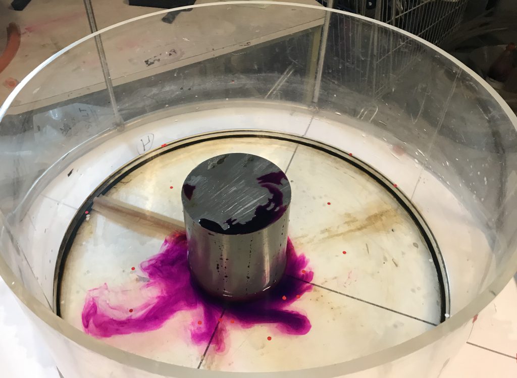
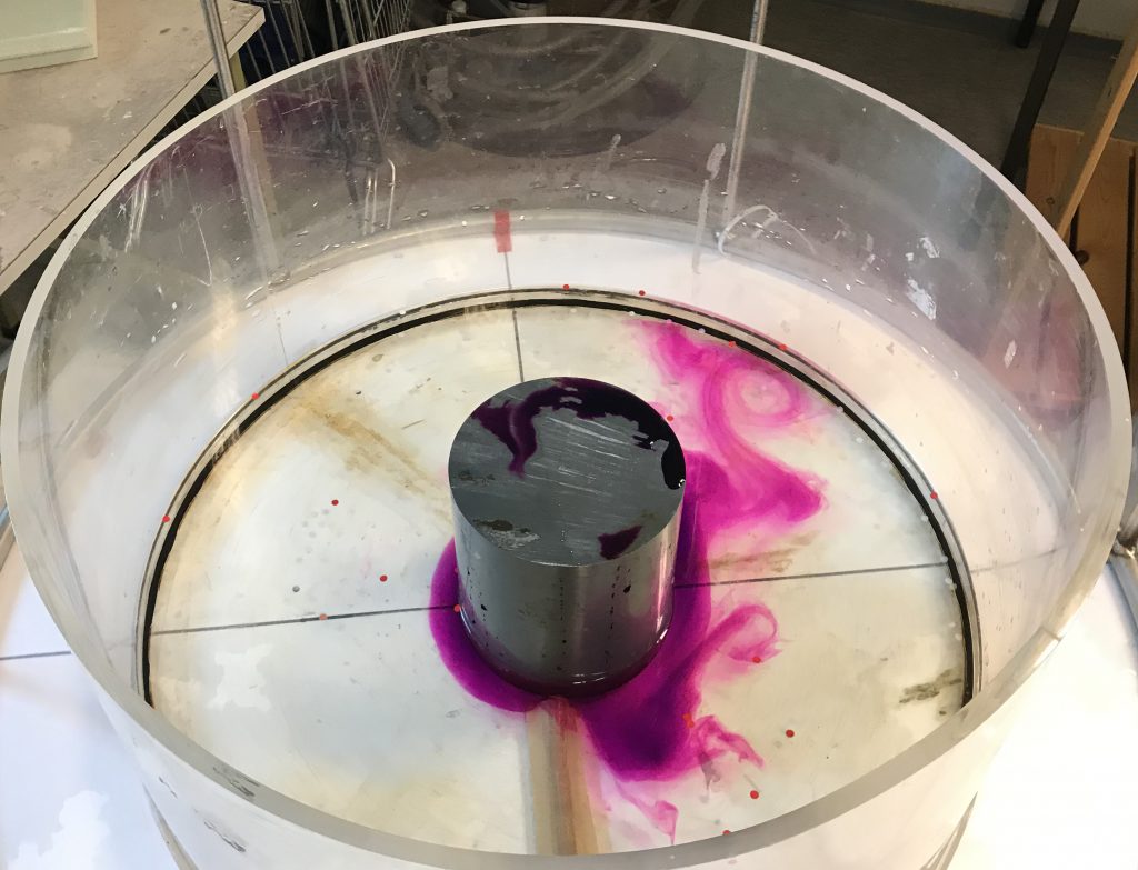
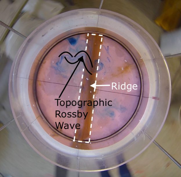
  • build a shallow ridge into the tank. They use an annulus and introduce the ridge at a random longitude, we could also build one across the center of the tank all the way to both sides to avoid weird things happening in the middle (or introduce a cylinder in the middle to mimic their annulus)
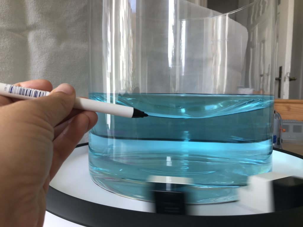
  • spin up the tank to approximately 26 rpm (that seems very fast! But that’s probably needed in order to create a parabolic surface with large height differences)
  • wait for it to reach solid body rotation (ca 10 min)
  • reduce rotation slightly, to approximately 23 rpm so the water inside the tank moves relative to the tank itself, and thus has to cross the ridge which is fixed to the tank
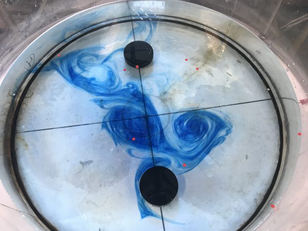
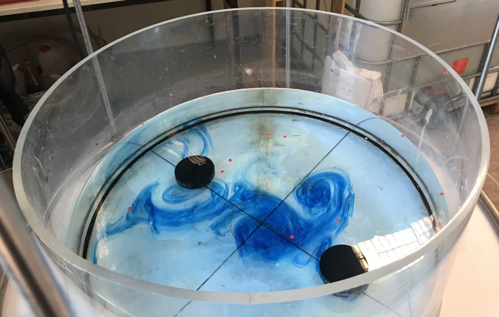
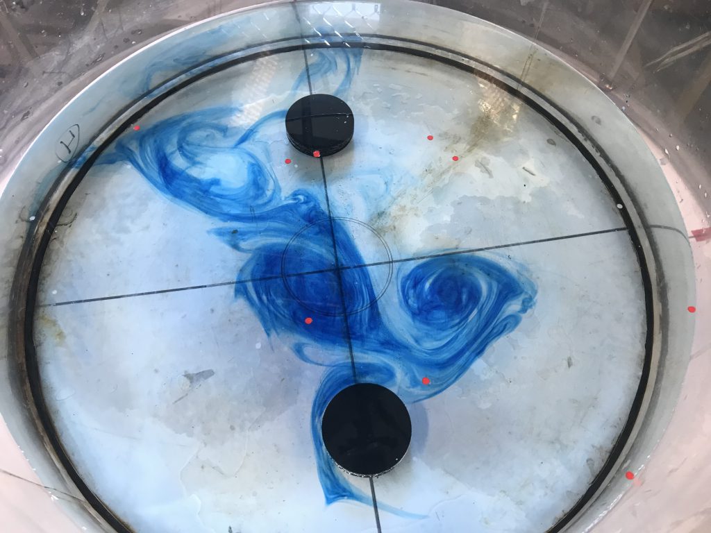
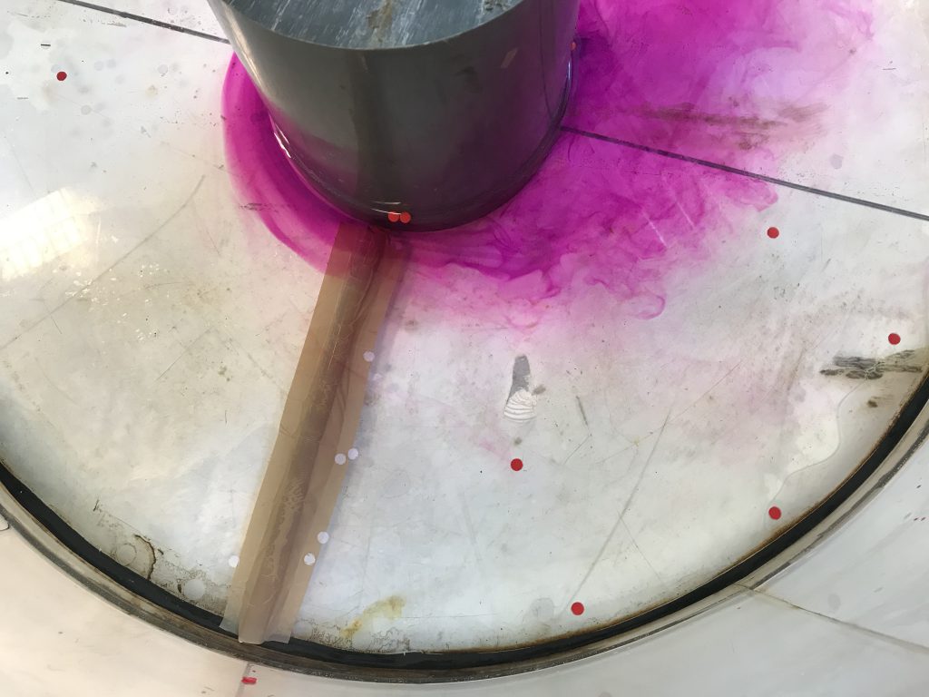
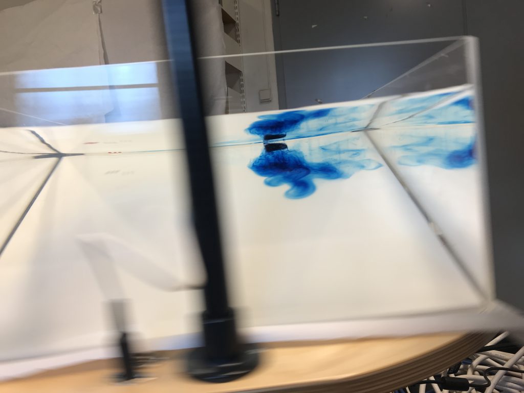
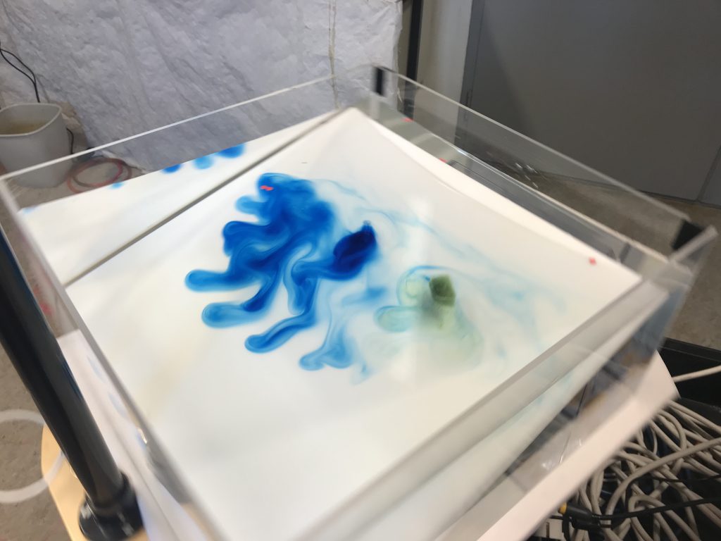
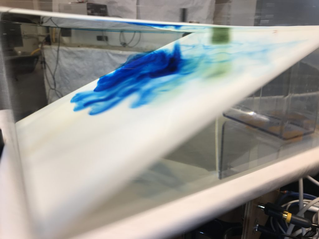
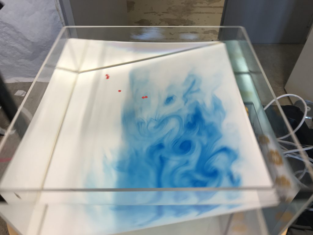
  • introduce dye upstream of the ridge, watch it change from laminar flow to eddies downstream of the ridge (they introduced dye at the inner wall of their annulus when the water was in solid body rotation, before slowing down the tank).

What are we expecting to see?

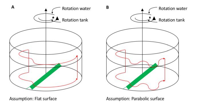
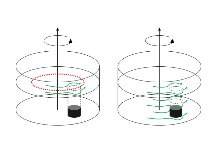
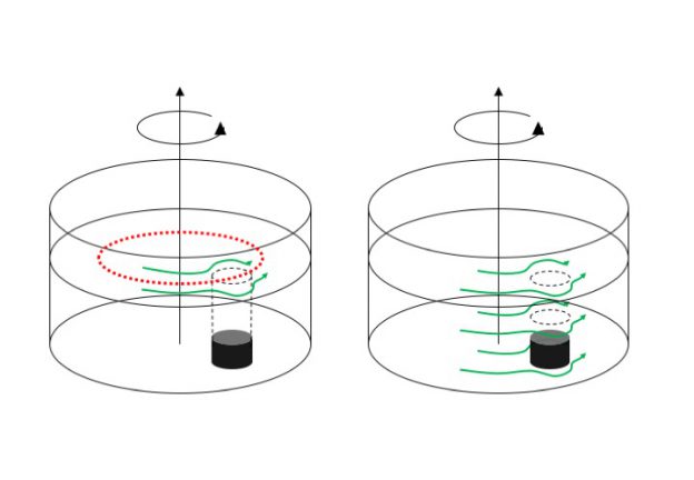
In case A, we assume that the rotation of the tank is slow enough that the surface is more or less flat. This will certainly not be the case if we rotate at 26rpm, but let’s discuss this case first, anyway. If we inject dye upstream of the obstacle, the dye will show that the current is being deflected as it crosses the ridge, to one direction as the water columns are getting shorter as they move up the ridge, then to the other direction when the columns are stretched going down the obstacle again. Afterwards, since the water depth stays constant, they would just resume a circular path.

In case B, however, we assume a parabolic surface of the tank, which we will have for any kind of fast-ish rotation. Initially, the current will move similarly to case A. But once it leaves the ridge, if it has any momentum in radial direction at all, it will overshoot its circular path, moving into water with a different depth. This will then again expand or compress the columns, inducing relative vorticity, leading to a meandering current and eddies downstream of the obstacle (probably a lot more chaotic than drawn in my sketch).

So in both cases we initially force the Rossby wave by topography at the bottom of the tank, but then in case B we sustain it by the changes in water depth due to the sloping surface.

My assessment before actually having run the experiment: The ridge seems fairly easy to construct and the experiment easy enough to run. However what I am worried about is the change in rotation rate and the turbulence and Ekman layers that it will introduce. After all, slowing down the tank is what we do create both turbulence and Ekman layers in demonstrations, and then we don’t even have an obstacle stuck in the tank. The instructions suggest a very slight reduction in rotation, so we’ll see how that goes…

Planetary Rossby waves on beta-plane

If we want to have more dramatic changes in water depth H than relying on the parabolic shape of the surface, another option is to use a rectangular tank and insert a sloping bottom as suggested by the Weather in a Tank group here. We are now operating on a Beta plane with the Coriolis parameter f being the sum of the tank’s rotation and the slope of the bottom.

Following the Weather in a Tank instructions, we plan to

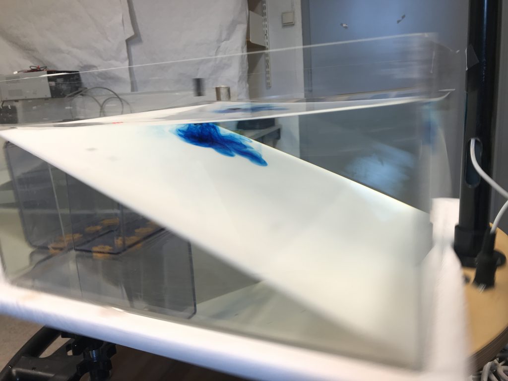
  • fill a tank with a sloping bottom (slope approximately 0.5)
  • spin it at approximately 15 rpm until it reaches solid body rotation (15-20 minutes later)
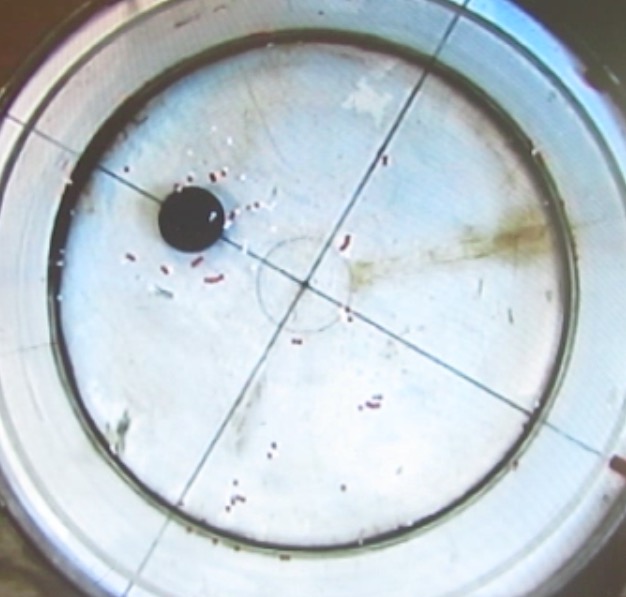
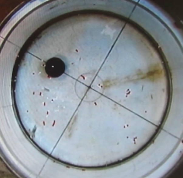
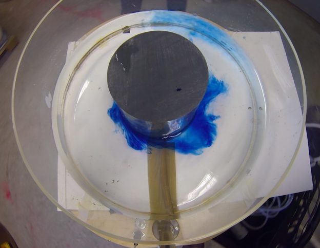
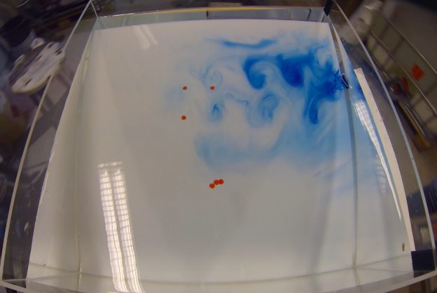
  • place a dyed ice cube (diameter approximately 5 cm) in the north-eastern corner of the tank

What do we expect to see?

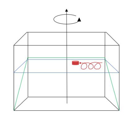
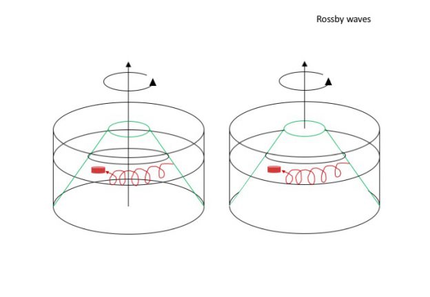
Ice cube and its trajectory (in red) on a sloping bottom in a rotating tank. Note: This sketch does not include the melt water water column!

Above is a simplified sketch of what will (hopefully!) happen. As the ice cube starts melting, melt water is going to sink down towards the sloping bottom, stretching the water column. This induces positive relative vorticity, making the water column spin cyclonically. As the meltwater reaches the sloping bottom, it will flow downhill, further stretching the water column. This induces more positive relative vorticity still, so the water column, and with it the ice cube, will start moving back up the slope until they reach the “latitude” at which the ice cube initially started. Having moved up the slope into shallower water, the additional positive vorticity induced by the stretching as the water was flowing down the slope has now been lost again, so rather than spinning cyclonically in one spot, the trajectory is an extended cycloid.

My assessment here (before having run it): I find this experiment a little more unintuitive because there are the different components of stretching contributing to the changes in relative vorticity. And from the videos I’ve seen, we don’t really get a clear column moving, but there are cyclonic eddies in the boundary layer that are shed. So I think this might be more difficult to observe and interpret. But I am excited to try!

Planetary Rossby wave on a cone (cyclical beta-plane?)

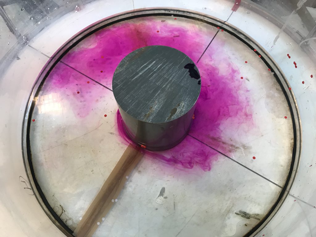
Following the Weather in a Tank instructions, we plan to also do the experiment as above but with cyclical boundary conditions, by using a cone in a cylindrical tank instead of a sloping bottom in a rectangular one.

The experiment is run in the same way as the one above (except they suggest a slightly slower rotation of 10 rpm). Physics are the same as before, except that now the transfer to reality should be a little easier, since we now have Rossby waves that can really run all the way around the pole. Also the experiment can be run for a longer time, since we don’t run into a boundary in the west if we are moving around and around the pole.

Ice cube and its trajectory (in red) on a cone in a rotating tank. Note: This sketch does not include the melt water column!

My assessment before actually having run the experiment: This shouldn’t be any more difficult to run, observe or interpret than the one above (at least once we’ve gotten our hands on a cone). Definitely want to try this!

Spin down — lots of shear instabilities in our tank!

When you stop a rotating tank, lots of stuff happens and it is usually very impressive to watch. Sometimes we stop tanks on purpose to show for example the development of Ekman layers, but sometimes we are just done with an experiment and then get to see cool stuff to see just as part of cleaning up.

Like below: When the tank stops, the water inside continues to spin, but friction with the sides and the bottom of the tank starts slowing the water down, inducing shear. Shear in turn produces turbulence and the structures cause smaller and smaller eddies. Very cool to watch!

Parabolic surface shape of a tank of water in solid body rotation

One of the first exercises Torge and I plan on doing with the students in our “dry theory to juicy reality” project is to bring a water-filled tank to solid body rotation and measure rotation, surface height at the center of the tank and the sides, as well as water depth before rotation, and then have them put those together according to theory.

Setup of the experiment as we did it using a glass vase my mom gave me as tank (diameter 24.5 cm). The non-rotating water depth was 9.2 cm. Once we rotated the tank with 10 rotations per 8.6 seconds, the maximum water level at the outside edge of the tank was approximately 10.8 cm, and the minimum 7.9 cm.

Seeing how difficult it is to “measure” the surface heights while the tank is rotating (we chose to draw circles on the outside of the tank at the heights where we thought the water levels were, in order to measure them later on a non-rotating tank), we were quite pleased with those results once we plugged them into the equations.

Calculating the resting water level as arithmetic mean between the rotating maximum value at the rim and the minimum value in the center, we are only off by 0.1 cm, so not too shabby!

And calculating the height difference between resting water level and rotating maximum level from the tangential velocity and radius of the tank, we are only off by 0.4 cm. So all in all, that’s working well!

Btw, below you see the resting water level and above the mark for the rotating maximum value. Quite impressive difference, isn’t it?

Anyway, looking at rotational surfaces and volumes and stuff this way is a lot more fun than doing it the dry theoretical way only! At least that’s what I think ;-)