This blog post was written for Elin Darelius & team’s blog (link). Check it out if you aren’t already following it!
—
I read a blog post by Clemens Spensberger over at a scisnack.com couple of years ago, where he talks about how ice can flow like ketchup. The argument that he makes is that ketchup on your hotdog behaves in many ways similarly to glaciers on for example Greenland: If there is a layer of a certain thickness, it will start sliding off — both the ketchup off your hotdog and the glaciers off Greenland. After most of it has dripped to your shirt or in the ocean, a little bit still remains on the hotdog or the mountain. And so on.
What he is talking about, basically, are effects of viscosity. Water, for example, would behave very differently than ketchup or ice, if you imagine it poured on your hotdog or raining down on Greenland. But also ketchup would behave very differently from ice, if it was put on Greenland in the same quantities as the existing glaciers on Greenland, instead of on a hotdog as a model version of Greenland in a relatively small quantity. And if you used real ice to model the behaviour of Greenland glaciers on a desk, then you would quickly find out that the ice just slides off on a layer of melt water and behaves nothing like you imagined (ask me how I know…).
This shows that it is important to think about what role viscosity plays when you set up a model. And not only when you are thinking about ice — also effects of surface tension in water become very important if your model is small enough, whereas they are negligible for large scale flows in the ocean.
The effects of viscosity can be estimated using the Reynolds number Re. Re compares the effects of the velocity u of the flow, a length scale of an obstacle L, and the viscosity v: Re = uL/v.
Reynolds numbers can be used to separate different flow regimes: laminar flows for very low Reynolds numbers, nice vortex streets for Re > 90, and then flows with a stagnant backwater for high Reynold numbers.
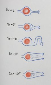
Dependency of a flow field on the Reynolds number. Shown is the top view of a flow field. You see red obstacles and blue stream lines (so any particle released at any point of a blue line would follow that line exactly, and in the direction shown by the arrow heads)
I have thought long and hard about what I could give as a good example for what I am talking about. And then I remembered that I did an experiment on vortex streets on a plate a while back.
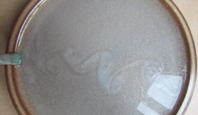
Vortices created on a plate
If you start watching the movie below at min 1:28 (although watching before won’t hurt, either) you see me pulling a paint brush across the plate at different speeds. The slow ones don’t create vortex streets, instead they show a more laminar behaviour (as they should, according to theory).
Vortex streets, like the one shown in the picture above, also exist in nature. However, scales are a lot larger there: See for example the picture below (Credit: Bob Cahalan, NASA GSFC, via Wikipedia)

Vortex street. Credit: Bob Cahalan, NASA GSFC, via Wikipedia
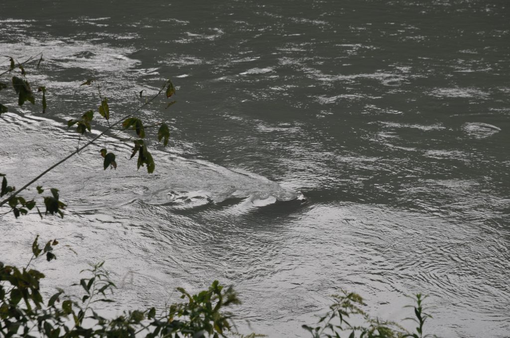
While this is a very distinctive flow that exists at a specific range of Reynolds numbers, you see flows of all different kinds of Reynold numbers in the real world, too, and not only on my plate. Below, for example, the Reynolds number is higher and the flow downstream of the obstacle distinctly more turbulent than in a vortex street. It’s a little difficult to compare it to the drawing of streamlines above, though, because the standing waves disguise the flow.
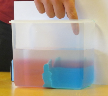
One way to manipulate the Reynolds number to achieve similarity between the real world and a model is to manipulate the viscosity. However that is not an easy task: if you wanted to scale down an ocean basin into a normal-sized tank, you would need fluids to replace the water that don’t even exist in nature in liquid form at reasonable temperatures.
All the more reason to use a large tank! :-)