Tag Archives: model

How can we use interactive flow simulations in teaching of hydrodynamics?

That was quite a teaser on Wednesday, wasn’t it? I said I had the solution to any hydrodynamics problem you might want to illustrate. So here we go:

I recently had the privilege to be given a private demonstration of the “Elbe” flow solver, which is being developed at Hamburg University of Technology. Elbe allows for near real time simulation of non-linear flows, and can be run in an interactive mode.

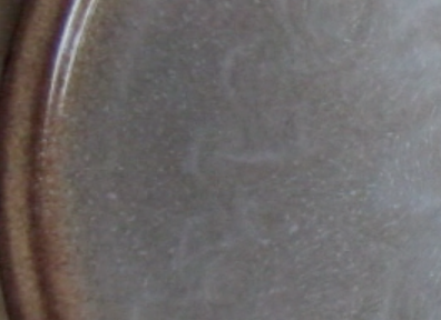
Look at the Karman vortex street below (their movie, not mine!) – doesn’t it remind you of the vortex street on a plate?

Now. How can we use such an awesome tool in teaching?

There are a couple of scenarios I could imagine.

1) Re-create flow fields.

This is mainly to help students get “a feel” for how a flow reacts to obstacles.

Provide students with a picture of a current field and ask them to recreate it as closely as possible. This is not about creating the exact same field, but about recognizing characteristics of a flow field and what might have caused them. Examples could include a Karman vortex street or a Kelvin Helmholtz instability.

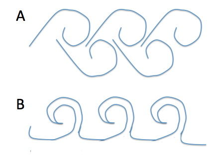
Possible sketches of A) Karman vortex street and B) Kelvin Helmholtz instabilities as examples for flow fields that students could be asked to recreate using Elbe.

In the above examples, students need to recognize, for example, that while a vortex street can be formed in a single-phase flow, a Kelvin Helmholtz instability typically forms on the boundary of layers of different densities in a shear flow (but could also form in a single continuous fluid), and recreate this in the model.

2) Visualize hydrodynamic concepts.

Here we would name a concept and ask students to set up a flow field that visualizes it. They might submit an annotated snapshot, for example. Possible examples are

– difference between stream lines, path lines and streak lines

– hydrodynamic paradox

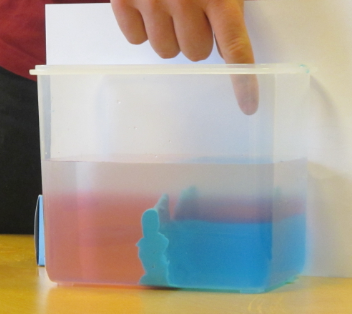
– dead water

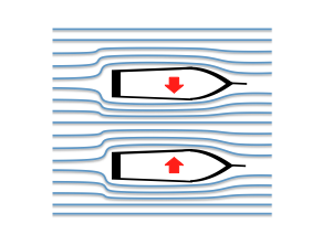
Hydrodynamic paradox. Moored ships are pulled towards each other because the flow is faster between them than upstream of them. (yes, the current in the picture is coming from the left, yet the ships are drawn as if the current was coming from the right. Shit happens.)

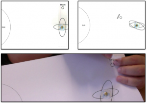
3) Test engineering applications.

Here we could imagine giving students different shapes and asking them to find their optimal position in a flow field, for example the pitch of a given wing profile to maximize lift, or the relative placement of a ship’s hull and a submerged ball for maximum canceling of waves.

4) Understanding of limitations of model and/or theory.

In some cases, students might be able to find optimal solutions from theory. In those cases it might be interesting to have them model those solutions and compare results with theoretical values. Can they come up with reasons why the modeled answers are likely different from the theoretical ones?

—

So far, so good. But how do we make sure that students don’t spend an insane amount of time fiddling with the nitty gritty details of the model, but focus on understanding hydrodynamics?

Combination of individual and group work

One idea might be to have students work individually on defining the important parameters (for example one- versus two-phase flow, obstacle at fixed position or moving, shape of obstacle) and then have them work in groups on putting those parameters into the model. If we were to grade this, we could give individual grades for individual answers to the first part, and then add a group grade in form of bonus points for a good model.

Model as a tool rather than the ultimate goal

Another idea would be to let them use the model as a tool rather than as the final application. As in students could be allowed to play with the model in order to, for example, figure out an approximate shape of an obstacle, and then they sketch their solution and annotate (e.g. “The longer X, the less turbulent region Y”). This would let them experience and explore hydrodynamics.

Peer-review

Whether or not a concept has been visualized well can be judged by the instructor, or it can become a learning activity in itself, for example as peer-review. Figuring out whether a visualization is correct or how it could be improved supports a deeper understanding of the concept as well as all kinds of interpersonal skills. In order to keep this interesting for students, several concepts could be visualized by different students and it can be made sure that the one students work on themselves is not the same as the one they will review later.

I am really excited to really start developing ideas on how to use this model in teaching. How would you use it?

Similarity requirements of a hydrodynamic model

1 Reply

Why downscaling only works down to a certain limit

When talking about oceanographic tank experiments that are designed to show features of the real ocean, many people hope for tiny model oceans in a tank, analogous to the landscapes in model train sets. Except even tinier (and cuter), of course, because the ocean is still pretty big and needs to fit in the tank.

What people hardly ever consider, though, is that purely geometrical downscaling cannot work. I’ve talked about surface tension a lot recently. Is that an important effect when looking at tides in the North Sea? Probably not. If your North Sea was scaled down to a 1 liter beaker, though, would you be able to see the concave surface? You bet. On the other hand, do you expect to see Meddies when running outflow experiments like this one? And even if you saw double diffusion happening in that experiment, would the scales be on scale to those of the real ocean? Obviously not. So clearly, there is a limit of scalability somewhere, and it is possible to determine where that limit is – with which parameters reality and a model behave similarly.

Mediterranean outflow. Mediterranean on the left, Atlantic Ocean on the right. The warm and salty water of the Mediterranean Outflow is dyed red.

I’ve noticed that people start glazing over when I talk about this, so in the future, instead of talking about it, I am going to refer them to this post. So here we go:

Similarity is achieved when the model conditions fulfill the three different types of similarity:

Geometrical similarity
Objects are called geometrically similar, if one object can be constructed from the other by uniformly scaling it (either shrinking or enlarging). In case of tank experiments, geometrical similarity has to be met for all parts of the experiment, i.e. the scaling factor from real structures/ships/basins/… to model structures/ships/basins/… has to be the same for all elements involved in a specific experiment. This also holds for other parameters like, for example, the elastic deformation of the model.

Kinematic similarity
Velocities are called similar if x, y and z velocity components in the model have the same ratio to each other as in the real application. This means that streamlines in the model and in the real case must be similar.

Dynamic similarity
If both geometrical similarity and kinematic similarity are given, dynamic similarity is achieved. This means that the ratio between different forces in the model is the same as the ratio between different scales in the real application. Forces that are of importance here are for example gravitational forces, surface forces, elastic forces, viscous forces and inertia forces.

Dimensionless numbers can be used to describe systems and check if the three similarities described above are met. In the case of the experiments presented on my blog, the Froude number and the Reynolds number are the most important dimensionless numbers.

The Froude number is the ratio between inertia and gravity. If model and real world application have the same Froude number, it is ensured that gravitational forces are correctly scaled.

The Reynolds number is the ratio between inertia and viscous forces. If model and real world application have the same Reynolds number, it is ensured that viscous forces are correctly scaled.

To obtain equality of Froude number and Reynolds number for a model with the scale 1:10, the kinematic viscosity of the fluid used to simulate water in the model has to be 3.5×10^-8m²/s, several orders of magnitude less than that of water, which is on the order of 1×10^-6m²/s.

There are a couple of other dimensionless numbers that can be relevant in other contexts than the kind of tank experiments we are doing here, like for example the Mach number (Ratio between inertia and elastic fluid forces; in our case not very important because the elasticity of water is very small) or the Weber number (the ration between inertia and surface tension forces). In hydrodynamic modeling in shipbuilding, the inclusion of cavitation is also important: The production and immediate destruction of small bubbles when water is subjected to rapid pressure changes, like for example at the propeller of a ship.

It is often impossible to achieve similarity in the strict sense in a model experiment. The further away from similarity the model is relative to the real worlds, the more difficult model results are to interpret with respect to what can be expected in the real world, and the more caution is needed when similar behavior is assumed despite the conditions for it not being met.

This is however not a problem: Tank experiments are still a great way of gaining insights into the physics of the ocean. One just has to design an experiment specifically for the one process one wants to observe, and keep in mind the limitations of each experimental setup as to not draw conclusions about other processes that might not be adequately represented.

Adventures in Oceanography and Teaching

Dr. Mirjam S. Glessmer

Tag Archives: model

How can we use interactive flow simulations in teaching of hydrodynamics?

Similarity requirements of a hydrodynamic model

A simple DIY tidal model