Tag Archives: Froude number

Playing with roll wave animations

I love how powerful Powerpoint is, at the same time there surely is a way out there to create these kind of animations with a little less copy & pasting, and especially without manually moving tons of stuff by juuust a tiny little bit from frame to frame?

How would you build these kinds of pictures? I’m even considering Matlab at this point (which I really don’t think would be such a stupid idea after all)

This is an animated gif. If it isn’t playing, I have no idea why not… It is playing on Twitter (link here)

Roll waves, one of the more complicated #friendlywaves I’ve gotten over the years…

#friendlywave is the new hashtag I am currently establishing. Send me your picture of waves, I will do my best to explain what’s going on there!

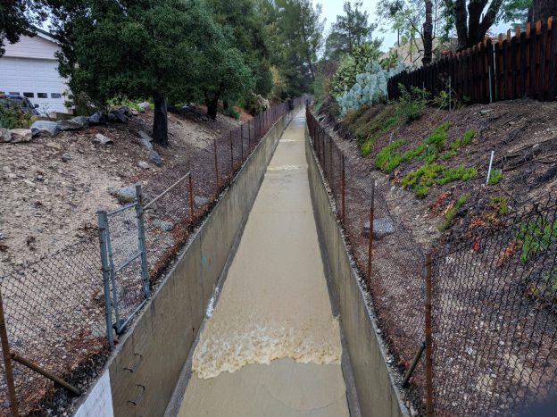
When it rains, it pours, especially in LA. So much so that they have flood control channels running throughout the city even though they are only needed a couple of days every year. But when they are needed, they should be a tourist attraction because of the awesome wave watching to be done there! As you see below, there are waves — with fronts perpendicular to the direction of flow and a jump in surface height — coming down the channel at pretty regular intervals.

Roll waves on Verdugo Wash. Photo by Mike Malaska

Even though this looks very familiar from how rain flows in gutters or even down window panes, having this #friendlywave sent to me was the first time I actually looked into these kinds of flows. Because what’s happening here is nothing like what happens in the open ocean, so many of the theories I am used to don’t actually apply here.

Looks like tidal bores traveling up a river

The waves in the picture above almost look like the tidal bores one might now from rivers like the Severn in the UK (I really want to go there bore watching some day!). Except that bores travel upstream and thus against the current, and in the picture both the flow and the waves are coming at us. But let’s look at tidal bores for a minute first anyway, because they are a good way to get into some of the concepts we’ll need later to understand roll waves, like for example the Froude number.

Froude number: Who’s faster, current or waves?

If you have a wave running up a river (as in: running against the current), there are several different scenarios, and the “Froude number” is often used to characterize them. The Froude number Fr=u/c compares how fast a current is flowing (u) with how fast a wave can propagate (c).


Side note: How do we know how fast the waves should be propagating?

The “c” that is usually used in calculating the Froude number is the phase velocity of shallow water waves c=sqrt(gH), which only depends on water depth H (and, as Mike would point out, on the gravitational constant g, which I don’t actually see as variable since I am used to working on Earth). (There is, btw, a fun experiment we did with students to learn about the phase speed of shallow water waves.) This is, however, a problem in our case since we are operating in very shallow water and the equation above assumes a sinusoidal surface, small amplitude and a lot of other stuff that is clearly not given in the see-saw waves we observe. And then this stuff quickly gets very non-linear… So using this Froude number definition is … questionable. Therefore the literature I’ve seen on the topic sometimes uses a different dispersion relation. But I like this one because it’s easy and works kinda well enough for my purposes (which is just to get a general idea of what’s going on).


Back to the Froude number.

If Fr<1 it means that the waves propagate faster than the river is flowing, so if you are standing next to the river wave watching, you will see the waves propagating upstream.

Find that hard to imagine? Imagine you are walking on an elevator, the wrong way round. The elevator is moving downward, you are trying to get upstairs anyway. But if you run faster than the elevator, you will eventually get up that way, too! This is what that looks like:

If Fr>1 however, the river is flowing faster than waves can propagate, so even though the waves are technically moving upstream when the water is used as a reference, an observer will see them moving downstream, albeit more slowly than the water itself, or a stick one might have thrown in.

On an escalator, this is what Fr>1 looks like:

But then there is a special case, in which Fr=1.

Hydraulic jumps

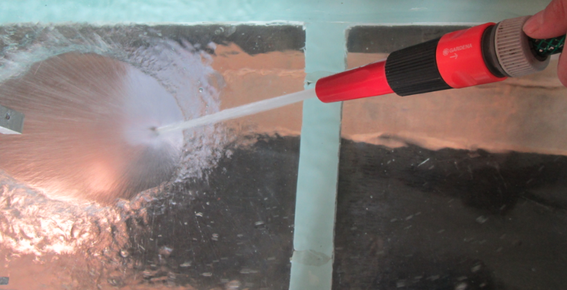
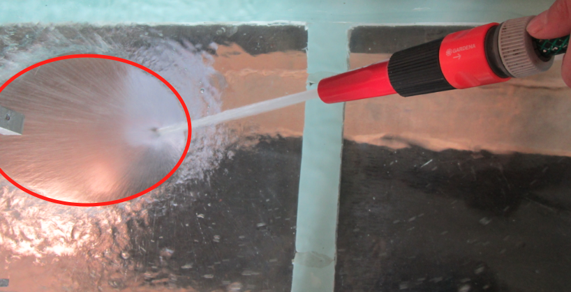
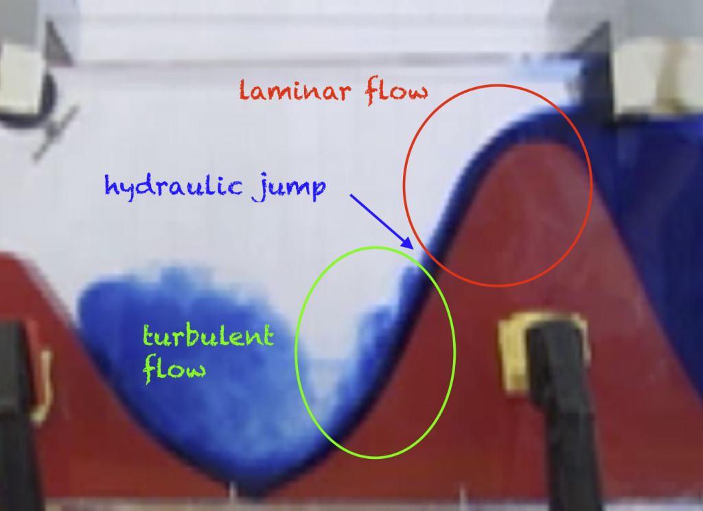
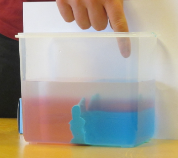
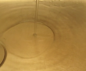
Fr=1 means that the current and the waves are moving at exactly the same velocity, so a wave is trapped in place. We see that a lot on weirs, for example, and there are plenty of posts on this blog where I’ve shown different examples of the so-called hydraulic jumps.

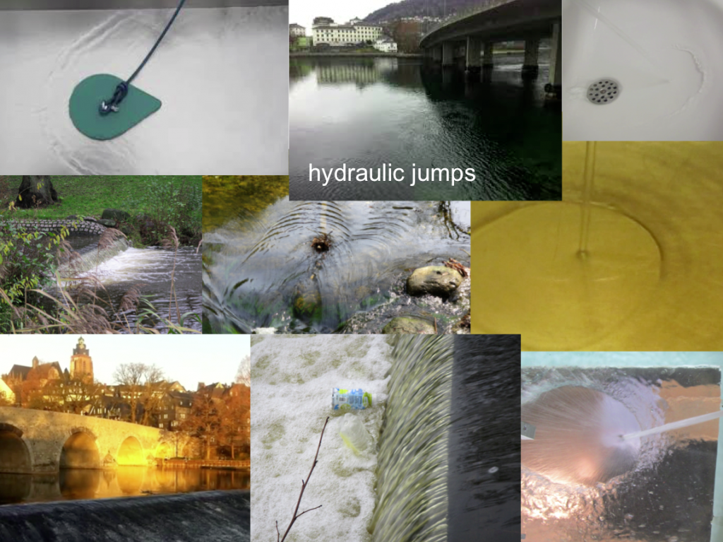
See? In all these pictures above there is one spot where the current is exactly as fast as the waves propagating against it, and in that spot the flow regime changes dramatically, and there is literally a jump in surface height, for example from shooting away from where the jet from the hose hits the bottom of the tank to flowing more slowly and in a thicker layer further out. However, all these hydraulic jumps stay in pretty much the same position over pretty long times. This is not what we observe with tidal bores.

On an escalator, you would be walking up and up and up, yet staying in place. Like so:

Roll waves

Tidal bores, and the hydraulic jumps associated with their leading edges, propagate upstream. But they are not waves the way we usually think about waves with particles moving in elliptical orbits. Instead, they are waves that are constantly breaking. And this is how they are able to move upstream: At their base, the wave is moving as fast as the river is flowing, i.e. Fr=1, so the base would stay put. As the base is constantly being pushed back downstream while running upstream at full force, the top of the wave is trying to move forward, too, moving over the base into the space where there is no base underneath it any more, hence collapsing forward. The top of the wave is able to move faster because it’s in “deeper” water and c is a function of depth. This is the breaking, the rolling of those waves. The front rolls up the rivers, entraining a lot of air, causing a lot of turbulent mixing as it is moving forward. And all in all, the whole thing looks fairly similar to what we saw in the picture above from Verdugo Wash.

But the waves are actually traveling DOWN the river

However there is a small issue that’s different. While tidal bores travel UP a river, the roll waves on Verdugo Wash actually travel DOWN. If the current and the waves are traveling in the same direction, what makes the waves break instead of just ride along on the current?

What’s tripping up these roll waves?

Any literature on the topic says that roll waves can occur for Fr>2, so any current that is twice as fast as the speed of waves at that water depth, or faster, will have those periodic surges coming downstream. But why? It doesn’t have the current pulling the base away from underneath it as it has in case of a wave traveling against the current, so what’s going on here? One thing is that roll waves occur on a slope rather than on a more or less level surface. Therefore the Froude number definitions for roll waves include the steepness of the slope — the steeper, the easier it is to trip up the waves.

Shock waves: Faster than the speed of sound

Usually shock waves are defined as disturbances that move faster than the local speed of sound in a medium, which means that it moves faster than information about its impending arrival can travel and thus there isn’t any interaction with a shock wave until it’s there and things change dramatically. This definition also works for waves traveling on the free surface of the water (rather than as a pressure wave inside the water), and describe what we see with those roll waves. Everything looks like business as usual until all of a sudden there is a jump in the surface elevation and a different flow regime surging past.

If you look at such a current (for example in the video below), you can clearly see that there are two different types of waves: The ones that behave the way you would expect (propagating with their normal wave speed [i.e. the “speed of sound”, c] while being washed downstream by the current) and then roll waves [i.e. “shock waves” with a breaking, rolling front] that surge down much faster and swallow up all the small waves in their large jump in surface elevation.

Video by Mike Malaska

In the escalator example, it would look something like this: People walking down with speed c, then someone tumbling down with speed 2c, collecting more and more people as he tumbles past. People upstream of the tumbling move more slowly (better be safe than sorry? No happy blue people were hurt in the production of the video below!).

Looking at that escalator clip, it’s also easy to imagine that wave lengths of roll waves become longer and longer the further downstream you go, because as they bump into “ordinary” waves when they are about to swallow them, they push them forward, thus extending their crest just a little more forward. And as the jump in surface height gets more pronounced over time and they collect more and more water in their crests, the bottom drag is losing more and more of its importance. Which means that the roll waves get faster and faster, the further they propagate downstream.

Speaking of bottom drag: When calculating the speed of roll waves, another variable that needs to be considered is the roughness of the ground. It’s easy to see that that would have an influence on shallow water. Explaining that is beyond this blog post, but there are examples in the videos Mike sent me, so I’ll write a blogpost on that soon.

So. This is what’s going on in LA when it is raining. Make sense so far? Great! Then we can move on to more posts on a couple of details that Mike noticed when observing the roll waves, like for example what happens to roll waves when two overflow channels run into each other and combine, or what happens when they hit an obstacle and get reflected.

Thanks for sharing your observations and getting me hooked on exploring this cool phenomenon, Mike!

Who is faster, the currents or the waves? The Froude number

A very convenient way to describe a flow system is by looking at its Froude number. The Froude number gives the ratio between the speed a fluid is moving at, and the phase velocity of waves travelling on that fluid. And if we want to represent some real world situation at a smaller scale in a tank, we need to have the same Froude numbers in the same regions of the flow.

For a very strong example of where a Froude number helps you to describe a flow, look at the picture below: We use a hose to fill a tank. The water shoots away from the point of impact, flowing so much faster than waves can travel that the surface there is flat. This means that the Froude number, defined as flow velocity devided by phase velocity, is larger than 1 close to the point of impact.

img_84791

At some point away from the point of impact, you see the flow changing quite drastically: the water level is a lot higher all of a sudden, and you see waves and other disturbances on it. This is where the phase velocity of waves becomes faster than the flow velocity, so disturbances don’t just get flushed away with the flow, but can actually exist and propagate whichever way they want. That’s where the Froude number changes from larger than 1 to smaller than 1, in what is called a hydraulic jump. This line is marked in red below, where waves are trapped and you see a marked jump in surface height. Do you see how useful the Froude number is to describe the two regimes on either side of the hydraulic jump?

img_84791-copy

Obviously, this is a very extreme example. But you also see them out in nature everywhere. Can you spot some in the picture below?

hydraulic_jumps

But still, all those examples are a little more drastic than what we would imagine is happening in the ocean. But there is one little detail that we didn’t talk about yet: Until now we have looked at Froude numbers and waves at the surface of whatever water we looked at. But the same thing can also happen inside the water, if there is a density stratification and we look at waves on the interface between water of different densities. Waves running on a density interface, however, move much more slowly than those on a free surface. If you are interested, you can have a look at that phenomenon here. But with waves running a lot slower, it’s easy to imagine that there are places in the ocean where the currents are actually moving faster than the waves on a density interface, isn’t it?

For an example of the explanatory power of the Froude number, you see a tank experiment we did a couple of years ago with Rolf Käse and Martin Vogt (link). There is actually a little too much going on in that tank for our purposes right now, but the ridge on the right can be interpreted as, for example, the Greenland-Scotland-Ridge, making the blue reservoir the deep waters of the Nordic Seas, and the blue water spilling over the ridge into the clear water the Denmark Strait Overflow. And in the tank you see that there is a laminar flow directly on top of the ridge and a little way down. And then, all of a sudden, the overflow plume starts mixing with the surrounding water in a turbulent flow. And the point in between those is the hydraulic jump, where the Froude number changes from below 1 to above 1.

screen-shot-2017-09-08-at-14-37-48-copy-e1504936264627

Nifty thing, this Froude number, isn’t it? And I hope you’ll start spotting hydraulic jumps every time you do the dishes or wash your hands now! :-)


Why we actually need a large tank — similarity requirements of a hydrodynamic model

When talking about oceanographic tank experiments that are designed to show features of the real ocean, many people hope for tiny model oceans in a tank, analogous to the landscapes in model train sets. Except even tinier (and cuter), of course, because the ocean is still pretty big and needs to fit in the tank.

What people hardly ever consider, though, is that purely geometrical downscaling cannot work. Consider, for example, surface tension. Is that an important effect when looking at tides in the North Sea? Probably not. If your North Sea was scaled down to a 1 liter beaker, though, would you be able to see the concave surface? You bet. On the other hand, do you expect to see Meddies when running outflow experiments like this one? And even if you saw double diffusion happening in that experiment, would the scales be on scale to those of the real ocean? Obviously not. So clearly, there is a limit of scalability somewhere, and it is possible to determine where that limit is – with which parameters reality and a model behave similarly.

Similarity is achieved when the model conditions fulfill the three different types of similarity:

Geometrical similarity
Objects are called geometrically similar, if one object can be constructed from the other by uniformly scaling it (either shrinking or enlarging). In case of tank experiments, geometrical similarity has to be met for all parts of the experiment, i.e. the scaling factor from real structures/ships/basins/… to model structures/ships/basins/… has to be the same for all elements involved in a specific experiment. This also holds for other parameters like, for example, the elastic deformation of the model.

Kinematic similarity
Velocities are called similar if x, y and z velocity components in the model have the same ratio to each other as in the real application. This means that streamlines in the model and in the real case must be similar.

Dynamic similarity
If both geometrical similarity and kinematic similarity are given, dynamic similarity is achieved. This means that the ratio between different forces in the model is the same as the ratio between different scales in the real application. Forces that are of importance here are for example gravitational forces, surface forces, elastic forces, viscous forces and inertia forces.

Dimensionless numbers can be used to describe systems and check if the three similarities described above are met. In the case of the experiments we talk about here, the Froude number and the Reynolds number are the most important dimensionless numbers. We will talk about each of those individually in future posts, but in a nutshell:

The Froude number is the ratio between inertia and gravity. If model and real world application have the same Froude number, it is ensured that gravitational forces are correctly scaled.

The Reynolds number is the ratio between inertia and viscous forces. If model and real world application have the same Reynolds number, it is ensured that viscous forces are correctly scaled.

To obtain equality of Froude number and Reynolds number for a model with the scale 1:10, the kinematic viscosity of the fluid used to simulate water in the model has to be 3.5×10⁻⁸m2/s, several orders of magnitude less than that of water, which is on the order of 1×10⁻⁶m2/s.

There are a couple of other dimensionless numbers that can be relevant in other contexts than the kind of tank experiments we are doing here, like for example the Mach number (Ratio between inertia and elastic fluid forces; in our case not very important because the elasticity of water is very small) or the Weber number (the ration between inertia and surface tension forces). In hydrodynamic modeling in shipbuilding, the inclusion of cavitation is also important: The production and immediate destruction of small bubbles when water is subjected to rapid pressure changes, like for example at the propeller of a ship.

It is often impossible to achieve similarity in the strict sense in a model experiment. The further away from similarity the model is relative to the real worlds, the more difficult model results are to interpret with respect to what can be expected in the real world, and the more caution is needed when similar behavior is assumed despite the conditions for it not being met.

This is however not a problem: Tank experiments are still a great way of gaining insights into the physics of the ocean. One just has to design an experiment specifically for the one process one wants to observe, and keep in mind the limitations of each experimental setup as to not draw conclusions about other processes that might not be adequately represented.

So much for today — we will talk about some of the dimensionless numbers mentioned in this post over the next weeks, but I have tried to come up with good examples and keep the theory to a minimum! :-)

Similarity requirements of a hydrodynamic model

Why downscaling only works down to a certain limit

When talking about oceanographic tank experiments that are designed to show features of the real ocean, many people hope for tiny model oceans in a tank, analogous to the landscapes in model train sets. Except even tinier (and cuter), of course, because the ocean is still pretty big and needs to fit in the tank.

What people hardly ever consider, though, is that purely geometrical downscaling cannot work. I’ve talked about surface tension a lot recently. Is that an important effect when looking at tides in the North Sea? Probably not. If your North Sea was scaled down to a 1 liter beaker, though, would you be able to see the concave surface? You bet. On the other hand, do you expect to see Meddies when running outflow experiments like this one? And even if you saw double diffusion happening in that experiment, would the scales be on scale to those of the real ocean? Obviously not. So clearly, there is a limit of scalability somewhere, and it is possible to determine where that limit is – with which parameters reality and a model behave similarly.

IMG_5320

Mediterranean outflow. Mediterranean on the left, Atlantic Ocean on the right. The warm and salty water of the Mediterranean Outflow is dyed red.

I’ve noticed that people start glazing over when I talk about this, so in the future, instead of talking about it, I am going to refer them to this post. So here we go:

Similarity is achieved when the model conditions fulfill the three different types of similarity:

Geometrical similarity
Objects are called geometrically similar, if one object can be constructed from the other by uniformly scaling it (either shrinking or enlarging). In case of tank experiments, geometrical similarity has to be met for all parts of the experiment, i.e. the scaling factor from real structures/ships/basins/… to model structures/ships/basins/… has to be the same for all elements involved in a specific experiment. This also holds for other parameters like, for example, the elastic deformation of the model.

Kinematic similarity
Velocities are called similar if x, y and z velocity components in the model have the same ratio to each other as in the real application. This means that streamlines in the model and in the real case must be similar.

Dynamic similarity
If both geometrical similarity and kinematic similarity are given, dynamic similarity is achieved. This means that the ratio between different forces in the model is the same as the ratio between different scales in the real application. Forces that are of importance here are for example gravitational forces, surface forces, elastic forces, viscous forces and inertia forces.


Dimensionless numbers can be used to describe systems and check if the three similarities described above are met. In the case of the experiments presented on my blog, the Froude number and the Reynolds number are the most important dimensionless numbers.

The Froude number is the ratio between inertia and gravity. If model and real world application have the same Froude number, it is ensured that gravitational forces are correctly scaled.

The Reynolds number is the ratio between inertia and viscous forces. If model and real world application have the same Reynolds number, it is ensured that viscous forces are correctly scaled.

To obtain equality of Froude number and Reynolds number for a model with the scale 1:10, the kinematic viscosity of the fluid used to simulate water in the model has to be 3.5×10⁻⁸m2/s, several orders of magnitude less than that of water, which is on the order of 1×10⁻⁶m2/s.

There are a couple of other dimensionless numbers that can be relevant in other contexts than the kind of tank experiments we are doing here, like for example the Mach number (Ratio between inertia and elastic fluid forces; in our case not very important because the elasticity of water is very small) or the Weber number (the ration between inertia and surface tension forces). In hydrodynamic modeling in shipbuilding, the inclusion of cavitation is also important: The production and immediate destruction of small bubbles when water is subjected to rapid pressure changes, like for example at the propeller of a ship.

It is often impossible to achieve similarity in the strict sense in a model experiment. The further away from similarity the model is relative to the real worlds, the more difficult model results are to interpret with respect to what can be expected in the real world, and the more caution is needed when similar behavior is assumed despite the conditions for it not being met.

This is however not a problem: Tank experiments are still a great way of gaining insights into the physics of the ocean. One just has to design an experiment specifically for the one process one wants to observe, and keep in mind the limitations of each experimental setup as to not draw conclusions about other processes that might not be adequately represented.

Hydraulic jump II

More movies of my kitchen sink.

I am really fascinated by the hydraulic jumps in my kitchen sink. I can’t believe I haven’t used this before when I was teaching! Yes, movies of rivers and rapids are always really impressive, too, but how cool is it to be able to observe hydraulic jumps in your own sink? Let me remind you:

Hydraulic jump in my kitchen sink. Video here

So this is what happens when the water jet hits the (more or less) level bottom of the sink. But what would happen if it instead hit a slope?

Now, if I wasn’t working a full-time job, or if that job wasn’t completely unrelated to anything to do with hydraulic jumps, I would now proudly present movies of all kinds of hydraulic jumps on sloped surfaces. As it is, I can tell you that I have tons of ideas of where to go to make really nice movies, but for now this is all I can offer:

Yes, that is a chopping board in a sink. It shows really nicely how the hydraulic jump occurs closer to the point of impact of the jet as you go uphill (because the water slows down faster going in that direction than going downhill) and again how the radius depends on the flow speed of the jet. Stay tuned for a more elaborate post on this!

Hydraulic jumps

Water changing its velocity from above to below the critical velocity.

Recently in beautiful Wetzlar: The river Lahn flows through the city below the medieval cathedral at sunset. And I’m showing you this because we can observe a hydraulic jump!

A hydraulic jump occurs when water that was flowing faster than the critical speed suddenly slows down to below the critical speed. Some of its kinetic energy is converted to potential energy (see the higher surface levels of the turbulent part of the fluid {except in this example the water is flowing down a steep slope, so the higher levels are a bit tricky to observe}) and a lot of energy is lost to turbulence. A very nice example can be seen here:

As the water moves away from where the jet hits the sink, it slows down. Can you spot the hydraulic jump? Isn’t it cool to watch how it is pushed away if the flow rate is higher, and how it comes back again when the tap is slowly closed?

P.S.: Yes, I’m being very vague about what that critical speed might be. Stay tuned for a post on that, I’m working on it! Just had to share the Lahn movie :-)